Welcome to the first lesson of your machine learning course! We're beginning our journey with a crucial first step in any data-driven project: Exploratory Data Analysis (EDA). Before we can build sophisticated models, we must first understand our data. This initial exploration allows us to uncover patterns, spot anomalies, and form hypotheses that will guide our entire modeling process.
Today's lesson focuses on univariate analysis, which is the practice of examining variables one by one. You will learn how to visualize the distribution of a single variable to understand its fundamental properties. Specifically, we will cover how to create and interpret three essential plot types—histograms, density plots, and box plots—to identify a distribution's spread (variability), skewness (asymmetry), and modality (number of peaks).
Describing a Distribution's Shape
When we look at a variable's distribution, we're interested in its "shape." This shape gives us clues about the data's underlying properties. The main characteristics we look for are modality and skewness.
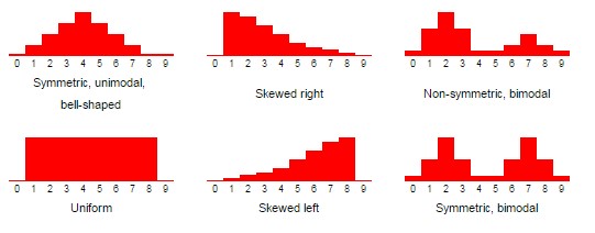
- Modality refers to the number of prominent peaks, or modes, in a distribution. A distribution can be unimodal (one peak), bimodal (two peaks), or multimodal (many peaks). A bimodal or multimodal distribution often suggests that the data contains distinct subgroups. A uniform distribution has no clear peaks.
- Skewness describes the asymmetry of the distribution. A symmetric distribution is balanced on both sides of its center, like the classic bell curve. A skewed distribution has a longer "tail" on one side.
- Right-skewed (or positively skewed): The long tail is on the right. The bulk of the data is concentrated on the left.
- Left-skewed (or negatively skewed): The long tail is on the left. The bulk of the data is concentrated on the right.
The image below shows several common distribution shapes you'll encounter.
Now, let's explore the tools we use to reveal these shapes from our data.
Tool 1: The Histogram
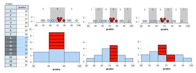
A histogram is one of the most common ways to visualize a distribution. It groups data into a series of intervals called "bins" and plots the frequency (the number of data points) within each bin as a bar. The height of the bar corresponds to the number of data points in that bin.
This is a great starting point for understanding a variable's distribution, but the visual representation is highly dependent on the number and width of the bins you choose.
Given your background, you'll find creating these plots in Python to be straightforward. The seaborn library, built on top of matplotlib, provides a high-level interface for creating statistically informative and aesthetically pleasing plots.
Tool 2: The Density Plot (KDE)
A density plot, or Kernel Density Estimate (KDE) plot, can be thought of as a smoothed histogram. Instead of using discrete bins, it represents the distribution with a continuous curve, which makes it excellent for observing the overall shape.
The y-axis of a density plot represents the probability density, not a direct frequency count. While the math behind it is complex, the intuition is simple: the height of the curve reflects the concentration of data points in that region. Higher peaks mean the data is more concentrated there.
Density plots are particularly useful for identifying modality and skewness without the distraction of bin selection.
To build a solid intuition for interpreting these plots, the following video offers a clear, conceptual overview.
How to interpret density plots - simple explanation with examples!
Watch this video from the Biostatsquid channel to understand how to interpret the key features of a density plot.
First, focus on the section explaining the shape of the curve, which covers symmetry, skewness, and modality. Then, watch the part that discusses variability, which explains how the width of the curve relates to the spread of the data.
Tool 3: The Box Plot
A box plot (or box-and-whisker plot) provides a compact summary of a distribution using five key numbers:
- Median (Q2): The line inside the box, representing the midpoint of the data.
- First Quartile (Q1): The bottom edge of the box (25th percentile).
- Third Quartile (Q3): The top edge of the box (75th percentile).
- The Box: Represents the Interquartile Range (IQR), which contains the middle 50% of the data. The length of the box is a measure of spread.
- Whiskers: These lines extend from the box to show the range of the rest of the data. By convention, they typically extend to 1.5 times the IQR from the box edges.
- Outliers: Any data points that fall outside the whiskers are plotted individually. This makes box plots excellent for outlier detection, a topic we will cover in detail later.
Box plots are less granular than histograms but are exceptional for quickly comparing the distributions of several groups side-by-side.
Creating and Interpreting the Plots
Now that you understand the concepts, let's see how they are applied. The following reading provides a practical guide to creating these visualizations in Python with seaborn and interpreting their output.
Assignment 4: Univariate data analysis — GEOG 30323
This guide by Kyle Walker provides a clear, code-driven introduction to univariate visualization using Python's seaborn library. It will walk you through creating and interpreting the plots we've just discussed.
Start by reading the section on univariate visualization. Then, work through the following subsections: Histograms: Read from the introduction to histograms to the exercise. This covers creating histograms with both pandas and seaborn's histplot function and interpreting their shape, including skewness and kurtosis. Density Plots: Continue to the section on kernel density plots, which shows how to create them with kdeplot and displot. Box Plots: Next, review the section on box plots. This explains how a box plot's components relate to a distribution's quartiles and how to spot outliers. Violin Plots: Finally, read the brief section on violin plots. A violin plot is a powerful hybrid that combines the features of a box plot with a density plot, giving you a view of both the summary statistics and the full distribution shape.
To reinforce these concepts and see more examples of interpretation, the "100 Days of Machine Learning" guide offers a focused breakdown.
Day 18: In-Depth Analysis of Histograms and Box Plots in Python
This resource provides a structured explanation of how to interpret histograms and box plots, which will complement the practical guide you just read.
Focus on these two parts: Read the section on Interpreting Histograms, which clearly defines shape analysis (symmetry, skewness, modality) and the effect of bin width. Read the section on Interpreting Box Plots. This gives a concise definition of the central box, median, whiskers, and outliers.
To see these seaborn functions in action, the following video provides a quick, practical demonstration.
Seaborn Crash Course - Data Visualization in Python
This crash course from the NeuralNine channel demonstrates how to quickly generate various plots in seaborn.
Watch the segment on distribution plots, where the presenter demonstrates displot, histplot, and kdeplot for visualizing univariate distributions. Next, watch the section on categorical plots, which includes boxplot and violinplot, showing how they summarize distributions.
Summary of Key Takeaways
This lesson introduced you to the first and most fundamental step in data exploration: analyzing variables one at a time.
- Three Key Plots: You learned about histograms, density plots, and box plots as essential tools for visualizing univariate distributions.
- Interpreting Shape: The primary goal of these visualizations is to understand a variable's underlying distribution by identifying its key characteristics:
- Spread: How dispersed or concentrated is the data? The width of a histogram/density plot and the IQR/whisker length of a box plot help measure this.
- Skewness: Is the data symmetric, or does it have a long tail to the right (positive skew) or left (negative skew)?
- Modality: Does the distribution have one (unimodal), two (bimodal), or more peaks? Multiple modes may indicate distinct subgroups in your data.
- Choosing the Right Plot:
- Histograms are great for a first look but can be sensitive to bin selection.
- Density plots excel at showing the overall distribution shape smoothly.
- Box plots offer a concise summary, are great for comparing many groups, and are excellent for spotting outliers.
With these foundational visualization skills, you are now equipped to start making sense of any new dataset you encounter.
In our next lesson, we will move from univariate to bivariate analysis, where you'll learn to visualize the relationships between two variables using tools like scatter plots, pair plots, and correlation heatmaps.