Identifying Data Quality Issues

The Importance of Data Quality

The principle of "garbage in, garbage out" is especially true in machine learning. No matter how sophisticated an algorithm is, its performance will be poor if the underlying data is flawed. Exploratory Data Analysis (EDA) is our first line of defense, allowing us to proactively detect these issues before they compromise our models.

The following video provides an excellent overview of why EDA is a critical first step, framing it as a process for understanding data, assisting with cleaning, and uncovering relationships.

We will focus on three key types of data issues that EDA helps us uncover. Let's dive in.

1. Identifying Missing Values

Missing values, often represented as NaN (Not a Number) in pandas, are gaps in your dataset where data was not collected or was lost. Most machine learning algorithms cannot process data with missing values, so identifying them is a mandatory first step.

Programmatic and Visual Detection

You can get a quick count of missing values per column using pandas. However, to understand the pattern of missingness, a visual approach is often more powerful. A heatmap can instantly show you which columns have missing data and whether there are any rows with multiple missing entries.

The following article from KDnuggets presents a series of practical Python techniques for EDA. We'll use it as a guide, starting with its method for detecting missing values. It also provides a handy synthetic dataset with pre-injected data issues that we can use for practice.

After running the code, you should see a visualization similar to this one:

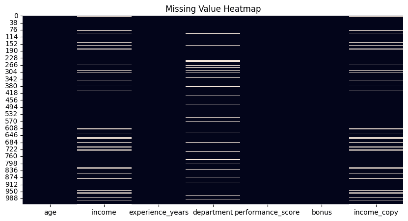
This visual approach is powerful because it can reveal patterns. For example, if you see that missing values in two columns often occur in the same rows, it might suggest a systematic reason for the data loss.

2. Identifying Outliers

Outliers are data points that deviate significantly from the rest of the observations. They can be genuine extreme values (e.g., a CEO's salary in an employee dataset) or errors (e.g., a human height of 20 feet). They are important because they can skew statistical measures and disproportionately affect the performance of many machine learning models.

Visual Detection with Box Plots

In our first lesson, you learned about box plots for univariate analysis. They are also an excellent tool for outlier detection. The "whiskers" of the plot define the expected range of the data, and any points that fall outside these whiskers are flagged as potential outliers.

The Data Analytics Lab video you watched earlier has a great segment on this.

Statistical Detection with the Interquartile Range (IQR) Method

The visual intuition of a box plot is formalized by the Interquartile Range (IQR) method. This is a robust statistical technique for flagging outliers. Here's the logic:

1. Find Quartiles: Calculate the first quartile (Q1, the 25th percentile) and the third quartile (Q3, the 75th percentile).
2. Calculate IQR: The IQR is the range between these quartiles: $IQR=Q3-Q1$.
3. Define Fences: Create "fences" or limits for our data. The standard rule is to place them 1.5 times the IQR below Q1 and above Q3.
   • Lower Fence: $Q1-1.5\times IQR$
   • Upper Fence: $Q3+1.5\times IQR$
4. Identify Outliers: Any data point that falls below the lower fence or above the upper fence is considered an outlier.

The following video from the codebasics channel provides an exceptionally clear explanation of this theory and its implementation in Python.

You can now apply this logic to the synthetic dataset from the KDnuggets article. The article itself provides a convenient function in Trick #3 that encapsulates this process. Try using it to find outliers in the 'income' column of the df you created.

3. Identifying Class Imbalance

Class imbalance occurs in classification problems when the different classes are not equally represented. For instance, in a dataset for fraud detection, the number of non-fraudulent transactions (majority class) will vastly outnumber fraudulent ones (minority class).

This is a problem because most machine learning models are optimized for accuracy. A naive model can achieve 99% accuracy on a dataset with a 99:1 class split by simply always predicting the majority class, making it useless for detecting the rare, important events.

Identifying Imbalance with Value Counts

Identifying class imbalance is straightforward. You can use the .value_counts() method on your target variable's column in pandas to see the distribution. A bar plot or seaborn.countplot of these values provides an immediate visual confirmation.

The following article from Analytics Vidhya explains why class imbalance is a critical issue and how to spot it.

In future lessons, we will cover techniques to handle this, such as over-sampling the minority class or under-sampling the majority class. For example, a common technique called SMOTE (Synthetic Minority Over-sampling Technique) generates new, synthetic examples of the minority class to create a balanced dataset.

For now, the key is simply to be able to identify that the problem exists in your dataset by checking the distribution of your target variable.

Conclusion

In this lesson, you've taken a major step in the data preprocessing journey by learning to diagnose critical data quality issues. You now have the skills to move beyond simple exploration and begin to critically evaluate your data's fitness for machine learning.

Here are the key takeaways:

• Data Quality is Paramount: The quality of your data directly dictates the quality of your model's predictions.
• Missing Values: Identify these using df.isnull().sum() for a numerical summary and a seaborn.heatmap of df.isnull() for a powerful visual overview of their patterns.
• Outliers: Detect these visually using box plots and statistically using the IQR method, which defines a valid data range using fences set at $Q1-1.5\times IQR$ and $Q3+1.5\times IQR$.
• Class Imbalance: In classification tasks, always check your target variable's distribution using .value_counts(). A significant skew between classes can make accuracy a misleading metric and requires special handling.

Now that you can identify these issues, our next lessons will focus on how to fix them. We will begin by exploring the common patterns of missing data and discussing various strategies to handle them, such as deletion and imputation.