Calculating and Interpreting Covariance

The Core Idea: Measuring How Variables Change Together

In the last lesson, we described a positive relationship as one where an increase in one variable tends to correspond with an increase in the other. A negative relationship was the opposite. Covariance is the statistical tool that formalizes this idea. It measures the degree to which two variables change or "vary" together—their "co-variance."

The StatQuest video below provides an excellent, intuitive introduction to this concept. It visually demonstrates how paired measurements can reveal a positive trend, a negative trend, or no trend at all.

As the video shows, covariance gives us a number that is:

• Positive when the variables tend to increase or decrease together.
• Negative when one variable tends to increase as the other decreases.
• Zero when there is no linear relationship between them.

The Intuition Behind the Formula

To calculate covariance, we need a formula that captures this logic. How can we mathematically determine if data points are consistently in the "low-low" & "high-high" quadrants (positive relationship) or the "low-high" & "high-low" quadrants (negative relationship)?

The key is to look at each data point's position relative to the mean of each variable.
Let's define our variables as $X$ and $Y$, with means $\bar{x}$ and $\bar{y}$. For any data point $(x_i,y_i)$:

• If $x_i>\bar{x}$ and $y_i>\bar{y}$ (top-right quadrant), both deviations $(x_i-\bar{x})$ and $(y_i-\bar{y})$ are positive. Their product is positive.
• If $x_i<\bar{x}$ and $y_i<\bar{y}$ (bottom-left quadrant), both deviations are negative. Their product is also positive.
• If $x_i<\bar{x}$ and $y_i>\bar{y}$ (top-left quadrant), the deviations have opposite signs. Their product is negative.
• If $x_i>\bar{x}$ and $y_i<\bar{y}$ (bottom-right quadrant), the deviations again have opposite signs. Their product is negative.

Covariance is essentially the average of these products. If the positive products dominate, the covariance will be positive. If the negative products dominate, it will be negative.

The StatQuest video masterfully walks through this logic.

This geometric interpretation is also clearly illustrated in the following article.

The Formula and Calculation

Now that you have the intuition, let's look at the formal definitions. We distinguish between the covariance of an entire population and that of a sample. Given your work in data science will almost always involve samples, the sample covariance formula is the one you will use most often.

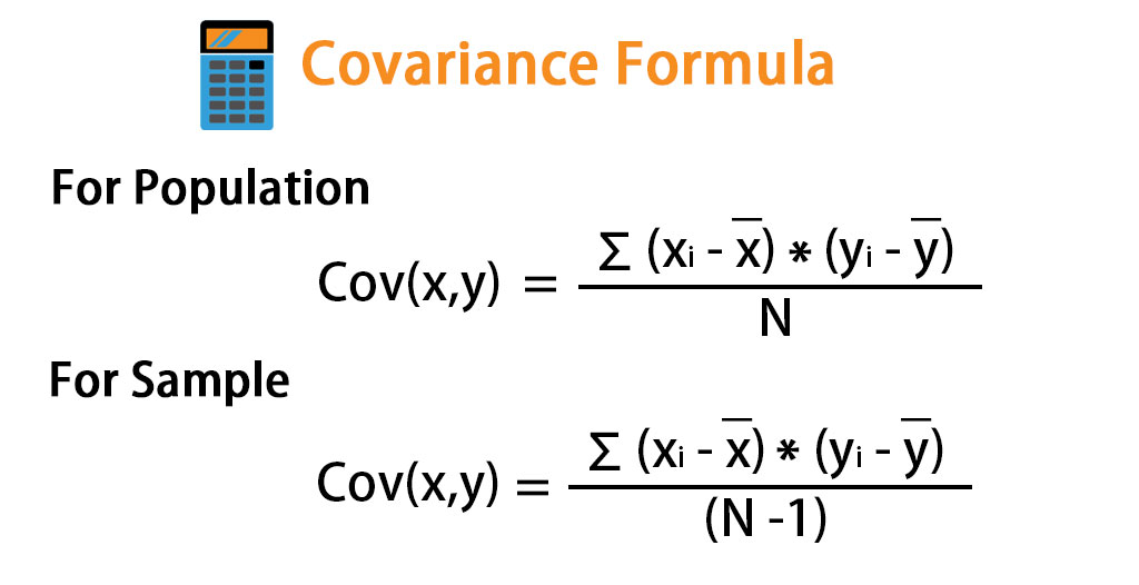
The sample covariance formula is:

Where:

• $x_i,y_i$ are the paired values of the variables.
• $\bar{x},\bar{y}$ are the sample means of each variable.
• $n$ is the number of data points in the sample.

Let's walk through a concrete example. The following video provides a clear, tabular method for performing the calculation by hand, which is an excellent way to ensure you understand every step of the process.

Interpreting the Covariance Value

After completing the calculation, you are left with a single number. What does it tell you?

1. The Sign: This is the most important piece of information.

   • Positive Covariance ($>0$): Indicates a positive linear relationship. As X increases, Y tends to increase.
   • Negative Covariance ($<0$): Indicates a negative linear relationship. As X increases, Y tends to decrease.
   • Zero Covariance ($=0$): Indicates no linear relationship. It's crucial to remember this doesn't rule out a non-linear relationship (e.g., a U-shape).

2. The Magnitude: This is where covariance has a major limitation. The absolute value of the covariance depends on the units of the variables themselves. For example, the covariance between height in meters and weight in kilograms will be much smaller than the covariance between height in centimeters and weight in grams, even if the underlying relationship is identical.

This makes it impossible to compare the strength of relationships across different datasets using covariance alone. A covariance of 50 might be very strong for one pair of variables but very weak for another.

The StatQuest and Organic Chemistry Tutor videos both do an excellent job of summarizing these points.

Covariance in Python

As a computer science student, you'll rarely calculate covariance by hand. In Python, the NumPy library makes this straightforward with the np.cov() function.

As the article explains, np.cov(x, y) returns a 2x2 covariance matrix:

• The values on the main diagonal are the variances of each variable. This makes sense, as the covariance of a variable with itself is its variance.
• The off-diagonal elements are the covariance between the two variables. The matrix is symmetric because $\text{Cov}(x,y)=\text{Cov}(y,x)$.

Understanding the structure of the covariance matrix is vital, as it is a fundamental component in many advanced statistical and machine learning techniques, such as Principal Component Analysis (PCA).

Conclusion

In this lesson, we have moved from visual inspection to numerical quantification of the relationship between two variables. We established a strong intuitive and mathematical understanding of covariance.

Key Takeaways:

• Covariance is a numerical measure of the direction of the linear relationship between two variables.
• A positive sign indicates that the variables tend to move in the same direction, while a negative sign indicates they move in opposite directions. A value of zero suggests no linear association.
• The calculation involves summing the product of deviations from the mean for each data pair and dividing by $n-1$ for a sample.
• The primary limitation of covariance is that its magnitude is dependent on the scale of the variables, making it difficult to interpret the strength of the relationship or compare it across different datasets.
• In Python, numpy.cov() returns a covariance matrix, where diagonal elements are variances and off-diagonal elements are the covariance.

The limitation of covariance naturally leads us to our next topic. We need a measure that is standardized, unit-free, and allows us to make meaningful comparisons about the strength of a linear relationship. This measure is the Pearson correlation coefficient, and it is what we will explore in the next lesson.