Scatter Plots: Visualizing Relationships

What is a Scatter Plot?

At its core, a scatter plot is a simple but powerful tool. It uses a two-dimensional Cartesian coordinate system to display the values of two quantitative variables from a dataset. Each point (or dot) on the plot represents a single observation or data point.

When we analyze the relationship between two variables, we often think in terms of cause and effect. We label the variable we believe might cause or explain the change as the explanatory variable (or independent variable) and place it on the horizontal x-axis. The variable that we expect to be affected is the response variable (or dependent variable), which goes on the vertical y-axis.

Let's begin by reading a short text that formally introduces these concepts.

To see how this works in practice, watch the first part of the following tutorial. It provides a very clear example using height and weight, and shows how to plot the first few points.

A Framework for Interpretation

Once you have your scatter plot, the real work of interpretation begins. Just looking at a cloud of dots isn't enough; we need a systematic way to describe what we see. A complete description of a scatter plot addresses four key characteristics: Direction, Form, Strength, and Outliers.

The same "Maths Tutorial" video provides a fantastic guide to each of these four elements. We'll go through it piece by piece.

First, watch the segment where the instructor introduces this four-part framework.

Now, let's break down each component.

1. Direction: Positive, Negative, or No Association

The direction describes the overall trend of the data as you read the plot from left to right.

• Positive Association: As the x-variable increases, the y-variable also tends to increase. The cloud of points slopes upwards from left to right.
• Negative Association: As the x-variable increases, the y-variable tends to decrease. The cloud of points slopes downwards from left to right.
• No Association: There is no discernible trend or slope. The points appear randomly scattered.

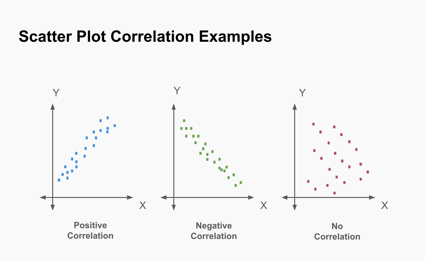
Watch the video segment below for a visual explanation.

2. Form: Linear or Non-linear

The form describes the shape of the pattern the dots create.

• Linear: The data points appear to cluster around a straight line. This is the most fundamental pattern we look for.
• Non-linear (or Curved): The data points follow a discernible pattern, but it's not a straight line. It could be a curve, a U-shape, or something more complex. If there's a clear pattern that isn't a straight line, it's crucial to note it.

3. Strength: Strong, Moderate, or Weak

Strength measures how closely the data points adhere to the form you identified. For a linear relationship:

• Strong: The points are tightly clustered around a line. The relationship is very clear.
• Moderate: The points are more spread out, but a general linear trend is still visible.
• Weak: The points are very scattered, and the linear trend is barely visible.
• Perfect: All points lie exactly on a single line (this is rare in real-world data).

4. Outliers

Outliers are individual data points that fall far from the overall pattern of the other points. They don't fit the general trend and can have a significant effect on numerical calculations. It's always important to identify them during visual inspection.

By describing these four characteristics, you can provide a comprehensive summary of the relationship shown in a scatter plot. For example, a good description might be: "There is a moderately strong, positive, linear relationship between variable X and variable Y, with one potential outlier in the upper-right corner."

Creating and Customizing Scatter Plots in Python

Now that we have a framework for interpretation, let's turn to the practical side. As a computer science student, you'll be creating these plots programmatically. The following video tutorial by Corey Schafer is an excellent, practical guide to creating scatter plots using the popular Python library matplotlib.

We'll start with the basics and then add layers of complexity and information.

The use of a log scale is a particularly important takeaway here. When dealing with data that spans several orders of magnitude (like view counts, income, or city populations), plotting on a linear scale can be misleading as a few large values will dominate the visual. A log scale helps to normalize the data and reveal trends that would otherwise be hidden.

Tying It All Together: A Final Example

Let's use our interpretation framework on a real-world scatter plot.

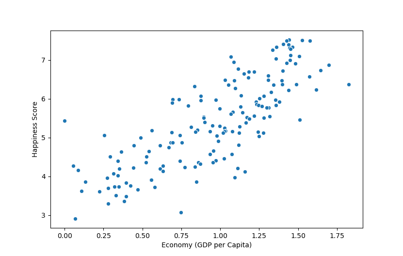
Let's analyze it using our four-part framework:

• Direction: The overall trend is positive. As a country's Economy (GDP per Capita) increases, its Happiness Score also tends to increase.
• Form: The relationship appears to be roughly linear. You could imagine drawing a straight line that captures the general trend. Some might argue there's a slight curve, where happiness gains diminish at higher GDP levels, which is also a valid observation.
• Strength: The strength is moderate. While there is a clear positive trend, the points are quite scattered. For any given GDP level, there is a wide range of happiness scores. This indicates that while GDP is a factor, it is far from the only factor determining happiness.
• Outliers: There are no extreme, glaring outliers that sit completely apart from the main cloud of points. However, you could identify countries that are "unusually" happy or unhappy for their GDP level by looking at points far above or below the main trend.

Conclusion

In this lesson, we took a deep dive into scatter plots, the cornerstone of visualizing relationships between two quantitative variables. You now have both a theoretical framework for interpretation and practical knowledge for creation.

Key Takeaways:

• Scatter plots visualize the relationship between an explanatory variable (x-axis) and a response variable (y-axis).
• A complete interpretation of a scatter plot involves describing its Direction (positive/negative), Form (linear/non-linear), Strength (strong/moderate/weak), and any Outliers.
• In Python, matplotlib provides powerful tools to not only create scatter plots but also customize them for clarity and to encode additional variables using color, size, and other aesthetics.
• Techniques like using a log scale are essential for dealing with real-world data that may have large outliers or span many orders of magnitude.

We have now learned how to see a relationship. However, "moderate" and "strong" are subjective terms. How can we put a number on the strength and direction of a linear relationship? That is precisely what our next lesson is about. We will introduce covariance and the Pearson correlation coefficient, the numerical measures that quantify what we have just learned to observe.