Pearson Correlation Coefficient: Calculation and Interpretation

Hello! In our last lesson, we explored covariance as a way to numerically describe the direction of a relationship between two variables. We concluded with its major limitation: the magnitude of covariance is dependent on the units of the data, making it impossible to judge the strength of a relationship or compare it across different datasets.

Today, we will build directly on that foundation to learn about the Pearson correlation coefficient, often denoted as $r$ . This is one of the most widely used statistics for measuring association. By the end of this lesson, you will be able to calculate this coefficient and, more importantly, interpret what its value tells us about the linear relationship between two variables. This resolves the core issue with covariance by providing a standardized, unit-less measure of both strength and direction.

From Covariance to Correlation

The conceptual leap from covariance to correlation is an elegant one. The Pearson correlation coefficient is simply the covariance of two variables, normalized by the product of their respective standard deviations.

The formula is:

r = \frac{Cov ( X , Y )}{σ _{X} σ _{Y}}

where $Cov (X, Y)$ is the covariance, and $σ_{X}$ and $σ_{Y}$ are the standard deviations of variables $X$ and $Y$ .

This act of dividing by the standard deviations is a form of standardization. It removes the influence of the variables' original scales and units. The result is a pure, dimensionless number that is always confined to the range of -1 to +1.

The following video from StatQuest provides an excellent explanation of why this normalization is so effective and what it achieves.

Pearson's Correlation, Clearly Explained!!!

This StatQuest video, "Pearson's Correlation, Clearly Explained!!!", will help you understand the intuition behind the formula.

Watch the segment that explains how the formula works, starting from the introduction of the formula. Pay close attention to the narrator's explanation of how the denominator "squeezes" the covariance into the -1 to 1 range.

Interpreting the Correlation Coefficient ( $r$ )

The value of $r$ gives us two key pieces of information:

The Sign (Direction):
- A positive $r$ indicates a positive linear relationship (as one variable increases, the other tends to increase).
- A negative $r$ indicates a negative linear relationship (as one variable increases, the other tends to decrease).
The Magnitude (Strength):
- An $r$ of +1 indicates a perfect positive linear relationship.
- An $r$ of -1 indicates a perfect negative linear relationship.
- An $r$ of 0 indicates no linear relationship.
- Values between 0 and $\pm 1$ describe the strength of the relationship. An $r$ of 0.8 represents a stronger linear relationship than an $r$ of 0.4.

The image below provides a fantastic visual summary of what different correlation values look like.

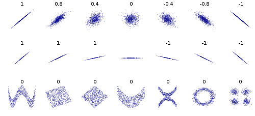
This last point is fundamental and cannot be overstated: Pearson's $r$ only measures the strength of a linear relationship. A low correlation does not necessarily mean there is no relationship between the variables; it just means there isn't a linear one. Always visualizing your data with a scatter plot is essential to avoid being misled by the $r$ value alone.

Calculating the Pearson Correlation Coefficient

While the conceptual formula $r = Cov (X, Y) / (σ_{X} σ_{Y})$ is best for understanding, for manual calculation, we typically expand it into one of two forms.

1. Definitional Formula (using deviations):
For a sample, this is written as:

r = \frac{\sum ( x _{i} - x ˉ ) ( y _{i} - y ˉ )}{\sum ( x _{i} - x ˉ ) ^{2} \sum ( y _{i} - y ˉ ) ^{2}}

You can see the components of covariance and variance directly in this formula. The numerator is the sum of cross-products of deviations (related to covariance), and the terms in the denominator are related to the standard deviations of $X$ and $Y$ .

2. Computational Formula (using sums):
This formula is algebraically equivalent but often easier for hand calculation as it doesn't require pre-calculating every deviation from the mean.

r = \frac{n ( \sum x y ) - ( \sum x ) ( \sum y )}{[ n \sum x ^{2} - ( \sum x ) ^{2} ] [ n \sum y ^{2} - ( \sum y ) ^{2} ]}

Here, $n$ is the number of data pairs. You simply need to calculate five sums from your data: $\sum x$ , $\sum y$ , $\sum x y$ , $\sum x^{2}$ , and $\sum y^{2}$ .

Let's walk through the calculation process.

Pearson Correlation Coefficient: Quantifying Relationships in Data

This DataCamp article provides a clear, step-by-step calculation using the definitional formula.

First, review the formula section to see how the conceptual and explicit formulas are presented. Then, follow the worked example for a small dataset of student study hours and exam scores. This will solidify your understanding of the calculation steps.

For a more detailed walkthrough using the computational formula, the following video is an excellent guide. It uses a clear, tabular method that is very systematic.

Correlation Coefficient

This video from The Organic Chemistry Tutor demonstrates the tabular method for calculating 'r'.

Watch from the start of the calculation. Follow along as the instructor: Creates a table with columns for x, y, xy, x^2, y^2. Calculates the required sums for each column. Plugs these sums into the computational formula to find the final r value.

Correlation in Practice: Python and Key Limitations

As a computer science student, you will almost always use a library to perform these calculations. In Python, the pandas and scipy libraries are standard.

Pearson Correlation Coefficient: Quantifying Relationships in Data

Let's return to the same DataCamp article to see how this is done in practice.

Read the section on calculating the coefficient in Python. Note the different functions available, particularly the .corr() method in pandas and pearsonr() in SciPy. The SciPy function is particularly useful as it also returns a p-value, a concept related to statistical significance that we will explore later in the course.

Understanding how to calculate $r$ is important, but knowing its limitations is what separates a novice from a proficient data analyst.

Pearson Correlation Coefficient: Quantifying Relationships in Data

Finally, let's look at how to interpret 'r' in context and its major limitations.

Read the section on interpreting the value, which discusses how the definition of a "strong" correlation can vary by field. Then, carefully read the section on the limitations of the coefficient. Pay special attention to the four points raised: correlation vs. causation, linearity, sensitivity to outliers, and restricted range.

Conclusion

In this lesson, we have taken the crucial step from the scale-dependent measure of covariance to the standardized, universally interpretable Pearson correlation coefficient.

Key Takeaways:

Pearson's correlation coefficient ( $r$ ) measures the strength and direction of a linear relationship between two quantitative variables.
It is calculated by normalizing the covariance by the product of the two variables' standard deviations, constraining its value to the range [-1, +1].
An $r$ value of 0 indicates no linear association, but it does not rule out the existence of a strong non-linear relationship. Visualizing data via scatter plots is non-negotiable.
The coefficient is sensitive to outliers and can be misleading if interpreted without context.

Perhaps the most critical limitation, and a mantra for any data scientist, is that correlation does not imply causation. Observing a strong correlation between two variables does not, on its own, allow us to conclude that one causes the other. In our next lesson, we will dedicate our time to exploring this vital distinction in detail, using examples to understand why this is the case and how lurking variables can create spurious correlations.

Recommended resources

From Covariance to Correlation

Interpreting the Correlation Coefficient (r)

Calculating the Pearson Correlation Coefficient

Correlation in Practice: Python and Key Limitations

Conclusion

Interpreting the Correlation Coefficient ( $r$ )