Understanding and Calculating Kurtosis

Hello! In our last lesson, we explored skewness, the third statistical moment, to quantify the asymmetry of a distribution. Today, we continue our journey into describing the shape of data by examining the fourth statistical moment. This leads us to the concept of kurtosis.

This lesson is designed to help you calculate kurtosis and, more importantly, interpret what it signifies about a distribution's tails and its propensity for outliers. While often introduced as a measure of "peakedness," you'll discover that its true statistical meaning is more nuanced and powerful, revolving around the weight of the tails. This understanding is critical in data science for identifying data characteristics that can heavily influence the performance of machine learning algorithms.

What is Kurtosis? Peakedness, Tails, and Outliers

Let's begin with the traditional, intuitive way kurtosis is often described: as the "peakedness" of a distribution. Imagine you have a standard bell curve. You could create a new distribution with the same mean and standard deviation by taking some data points from the "shoulders" of the curve and moving them to the center (making it more peaked) and to the far ends (making the tails heavier or "fatter"). Kurtosis is the measure that allows us to distinguish between these two distributions, which would otherwise seem similar based on their mean and variance.

The following video from zedstatistics provides an excellent visual introduction to this idea.

What is Kurtosis? (+ the "peakedness" controversy!)

This video, "What is Kurtosis?", starts by explaining the traditional view of kurtosis as 'peakedness' and the idea of redistributing mass from a distribution's shoulders to its peak and tails.

Watch the introductory segment from the beginning. Pay close attention to the visual of the white and black curves, which both have the same mean and standard deviation but differ in shape. This difference is what kurtosis aims to capture.

This idea gives us three general categories of distribution shapes related to kurtosis:

Leptokurtic: More peaked and with heavier tails than a normal distribution.
Mesokurtic: Having a peak and tails similar to a normal distribution.
Platykurtic: Flatter and with lighter tails than a normal distribution.

Let's look at some examples to make this more concrete.

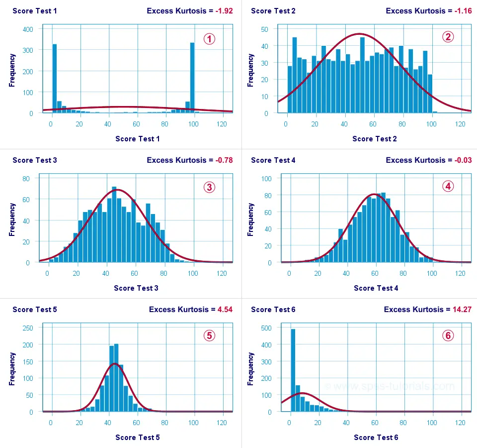
These six histograms show distributions with varying shapes and corresponding excess kurtosis values. A normal distribution serves as a reference curve.

In the "Examples of Kurtosis in Histograms" image above:

Test 4 is a nearly perfect bell shape. It's mesokurtic, and its excess kurtosis is close to 0.
Test 5 is more peaked in the center and has thinner shoulders than the normal curve. It's leptokurtic, with a positive excess kurtosis of 4.54.
Test 3 is flatter than the normal curve, with "heavier shoulders." It's platykurtic, with a negative excess kurtosis of -0.78. Notice how Test 1 (bimodal) and Test 2 (uniform) are even flatter, resulting in more negative kurtosis values.

The Real Story: Kurtosis Measures Tailedness

While "peakedness" is a helpful starting point, it's not the whole story. In fact, modern statistical understanding emphasizes that kurtosis is fundamentally a measure of tailedness—that is, the weight of the tails and the potential for a distribution to produce outliers.

The reason for this lies in the mathematical formula. As we will see, kurtosis is calculated using the fourth power of the distance of each data point from the mean. This means that points far from the mean (in the tails) have an exponentially larger impact on the kurtosis value than points near the center (in the peak). A single extreme outlier can dramatically increase the kurtosis of a dataset.

The following article by Gregory Gundersen provides a rigorous explanation, which will be valuable given your mathematical background. He convincingly argues that kurtosis is about tails, not peaks.

Understanding Moments

This article explains kurtosis as the fourth standardized moment and directly addresses the 'peakedness' misconception. It uses a clear example to show that the tail values dominate the kurtosis calculation.

Please read the section on Kurtosis. The Python code example is particularly illustrative; it demonstrates that for a Cauchy distribution (which is peaked and has heavy tails), nearly 100% of the kurtosis value comes from data points in the tails, not the peak.

The zedstatistics video also explores this "controversy," concluding that the modern interpretation focuses on tails and outliers.

What is Kurtosis? (+ the "peakedness" controversy!)

This final part of the video discusses the academic debate around kurtosis, concluding that its calculation is most sensitive to outliers and the thickness of the tails.

Watch the segment on the controversy. The explanation of how the fourth-power term in the formula amplifies the effect of outliers is the key takeaway here.

Calculating Kurtosis

Now let's formalize this. Just as skewness was the third standardized moment, kurtosis is the fourth standardized moment.

For a population, the formula is:

Kurtosis = E [(\frac{X - μ}{σ})^{4}] = \frac{μ _{4}}{σ ^{4}}

where $μ_{4}$ is the fourth central moment. This formula calculates the average of the standardized deviations raised to the fourth power.

Excess Kurtosis

A crucial fact in statistics is that a perfect normal distribution has a kurtosis value of 3. You can see the mathematical proof for this in Appendix A3 of the Gundersen article.

Because the normal distribution is such a common benchmark, it's often more convenient to compare other distributions to it. This gives rise to excess kurtosis:

Excess Kurtosis = Kurtosis - 3

By this definition:

A normal (mesokurtic) distribution has an excess kurtosis of 0.
A leptokurtic distribution (heavy tails) has an excess kurtosis > 0.
A platykurtic distribution (light tails) has an excess kurtosis < 0.

Important Note: Most statistical software packages (like SPSS, Excel, Python's scipy.stats) calculate excess kurtosis by default, but they often label it simply as "kurtosis." From now on, when we refer to kurtosis values, we will be talking about excess kurtosis unless stated otherwise.

The following resource walks through the formulas and provides a worked example.

Kurtosis (Statistics) - Quick Tutorial

This tutorial from SPSS-tutorials.com clearly lays out the formulas for population kurtosis, explains the shift to excess kurtosis, and shows a step-by-step calculation in a spreadsheet.

First, review the Kurtosis Formulas. Then, read the section Kurtosis or Excess Kurtosis? to solidify your understanding of this key distinction. Finally, walk through the Kurtosis Calculation Example to see how the numbers come together. You don't need to memorize the complex sample adjustment formula, but understand that it exists to make the sample statistic a better estimate of the population parameter.

Interpreting Kurtosis

With the calculations clear, let's focus on interpretation. The sign and magnitude of the excess kurtosis value tell us about the shape of our distribution's tails relative to a normal distribution.

These plots show the characteristic shapes of leptokurtic, mesokurtic, and platykurtic distributions. The density plot on the left highlights the peak and tail differences. The quantile-quantile (Q-Q) plot on the right shows how the tails deviate from a normal distribution.

The tutorial page from before gives us the formal terminology.

Kurtosis (Statistics) - Quick Tutorial

This section provides the formal definitions for the three types of kurtosis.

Read the brief section Platykurtic, Mesokurtic & Leptokurtic.

Here's a summary of how to interpret excess kurtosis values:

Excess Kurtosis > 0 (Leptokurtic): The distribution has heavier tails than a normal distribution. This suggests that outliers are more likely. Financial returns data, for example, are often leptokurtic, exhibiting more extreme price movements ("fat tails") than a normal distribution would predict.
Excess Kurtosis ≈ 0 (Mesokurtic): The distribution's tails are similar to a normal distribution. This is the baseline case.
Excess Kurtosis < 0 (Platykurtic): The distribution has lighter tails than a normal distribution. This means outliers are less likely. A uniform distribution is an example of a platykurtic distribution; it has no tails at all, as the data is constrained within a fixed range.

Conclusion

Today, we've completed our initial look at the shape of distributions by examining kurtosis. You have seen how it functions as the fourth statistical moment and, more importantly, what it reveals about a dataset.

Key Takeaways:

Kurtosis is the fourth standardized moment, and it measures a distribution's "tailedness."
While often associated with "peakedness," its value is primarily driven by the presence and extremity of outliers.
Excess Kurtosis subtracts 3 (the kurtosis of a normal distribution) to set the normal distribution as a baseline of 0.
A leptokurtic distribution (positive excess kurtosis) has heavy tails, indicating a higher probability of extreme values.
A platykurtic distribution (negative excess kurtosis) has light tails, indicating a lower probability of extreme values.

Having now covered measures of central tendency, dispersion, and shape (skewness and kurtosis), you have a robust toolkit for describing the characteristics of a single variable.

In our next lesson, we will shift our focus. Instead of describing one variable at a time, we will begin to explore the relationships between pairs of variables, starting with the fundamental concepts of covariance and correlation.