Hello! In our previous lessons, we've become proficient at finding quartiles, deciles, and percentiles to pinpoint the position of values within a dataset. Now, we'll use that skill to derive one of the most important measures of statistical spread.
This lesson focuses on calculating the interquartile range (IQR). You'll learn how to compute this value and, more importantly, understand what it tells us about the concentration of our data. The IQR is a measure of dispersion that describes the spread of the middle half of your dataset, making it a key tool in exploratory data analysis and a fundamental building block for visualizations like the boxplot.
Defining the Interquartile Range
While measures of central tendency like the median tell us about the center of our data, they don't describe its spread. The simplest measure of spread is the range (the difference between the maximum and minimum values). However, the range is highly sensitive to outliers—a single extremely high or low value can dramatically alter it.
The interquartile range (IQR) offers a more robust solution. It focuses on the spread of the middle 50% of the data, effectively ignoring the most extreme values in the lowest and highest 25%.
The formula is elegantly simple:
Where:
- Q3 is the third quartile (the 75th percentile).
- Q1 is the first quartile (the 25th percentile).
Because it discards the upper and lower quarters of the data, the IQR is not affected by outliers, making it a superior measure of spread for skewed distributions or datasets with anomalies. This property is sometimes referred to as having a high breakdown point; up to 25% of the data can be outliers without corrupting the IQR. The simple range, by contrast, has a breakdown point of 0%.
The Calculation Process
Calculating the IQR is a straightforward process that builds directly on our last two lessons.
- Order the Data: Arrange your dataset in ascending order.
- Find the Median (Q2): Locate the median of the entire dataset.
- Find Q1 and Q3:
- Identify the lower half of the data (all values to the left of the median). Q1 is the median of this lower half.
- Identify the upper half of the data (all values to the right of the median). Q3 is the median of this upper half.
- Calculate the IQR: Subtract the first quartile from the third quartile: .
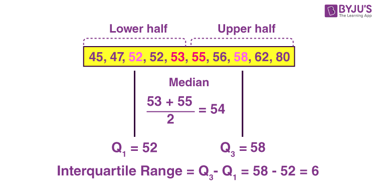
The following image provides a clear, step-by-step example for a dataset with an even number of points.
Nuances in Calculation: Inclusive vs. Exclusive Methods
A subtle but important point arises when the dataset has an odd number of values: what do we do with the median when splitting the data into lower and upper halves? This leads to two slightly different, but equally valid, methods. Your computer science background will appreciate that different algorithms can be used to solve the same problem, sometimes with minor differences in output.
- Exclusive Method: The median is excluded from both the lower and upper halves. This is the most common method taught in introductory statistics.
- Inclusive Method: The median is included in both the lower and upper halves.
While there's no universal consensus, the exclusive method is more prevalent. Different statistical software packages (like R, Python's pandas, or Excel) may use different underlying methods, which can lead to small variations in quartile and IQR calculations.
The following article from Scribbr provides an excellent, detailed explanation of these two methods with clear examples.
How to Find Interquartile Range (IQR) | Calculator & Examples
This article offers a comprehensive guide to calculating the IQR. It defines the concept and then clearly distinguishes between the "exclusive" and "inclusive" methods, which is crucial for understanding why results might vary between different statistical tools.
Start by reading the introduction and the section on the basic formula. Then, pay close attention to the section "Exclusive method vs inclusive method", as it explains the key difference in algorithms. Finally, walk through the step-by-step examples for the exclusive method and the inclusive method to see them in practice.
IQR Calculation in Action
Watching the calculation performed on a few datasets can help solidify the process. The video below demonstrates the "exclusive" method for both an odd-numbered and an even-numbered dataset.
How To Find The Interquartile Range & any Outliers - Descriptive Statistics
This video from The Organic Chemistry Tutor provides two clear, worked examples of finding the IQR. The first example has an odd number of data points, and the second has an even number, covering both scenarios you will encounter.
First, watch the example for an odd-numbered dataset from this segment. Notice how the median is identified and then excluded when finding Q1 and Q3. Next, watch the example for an even-numbered dataset starting at this point. Observe how the median is the average of the two central values, and how the data is split cleanly into two halves to find the quartiles.
Visualizing the Interquartile Range: The Boxplot
The IQR is not just an abstract number; it has a powerful visual representation in a boxplot (also known as a box-and-whisker plot). In a boxplot, the "box" itself represents the interquartile range.
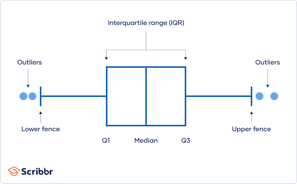
A wide box indicates a large IQR and high variability in the central part of the data. A narrow box signifies a small IQR and that the central data points are clustered closely together. We will explore boxplots in much more detail in a future lesson.
Conclusion
You have now added a crucial measure of dispersion to your statistical toolkit. The interquartile range provides a robust way to quantify the spread of your data, laying the groundwork for more advanced data analysis and visualization.
Key Takeaways:
- The Interquartile Range (IQR) is the difference between the third quartile (Q3) and the first quartile (Q1).
- It represents the spread of the middle 50% of the data.
- The IQR is a robust measure of spread, meaning it is not easily influenced by outliers, unlike the simple range.
- Minor variations in calculation methods (e.g., inclusive vs. exclusive) exist, which can lead to slightly different results in various software tools.
- The IQR is visually represented by the box in a boxplot.
In our next lesson, we will shift our focus from measures of position and spread to measures that describe the overall shape of a distribution. We'll explore statistical moments, which will allow us to quantify concepts like skewness (asymmetry) and kurtosis (the "tailedness" or peakiness) of our data.