Hello!
In our previous lessons, we built a comprehensive toolkit for describing a single variable using numerical summaries. We explored measures of central tendency (mean, median, mode), dispersion (variance, standard deviation), and shape (skewness, kurtosis). Now, we will begin our next major topic: Exploratory Data Analysis (EDA). EDA is the process of using summaries and visualizations to understand a dataset's main characteristics, uncover patterns, and spot anomalies before any formal modeling begins.
This lesson marks our first step into EDA by tackling a fundamental question: how can we take a raw, jumbled list of data points and organize it into a meaningful summary? We will answer this by learning how to construct and interpret frequency distribution tables. This technique is the bedrock for many of the data visualizations, like histograms, that we will cover next.
From Raw Data to Structured Insight
Imagine you have a list of 100 exam scores, 500 customer responses, or a million sensor readings. Simply looking at the raw numbers is overwhelming and uninformative. The first step in making sense of this data is to summarize it. A frequency distribution table, often just called a frequency table, is one of the simplest yet most powerful ways to do this.
It works by categorizing the data and counting how many observations fall into each category. This count is called the frequency.
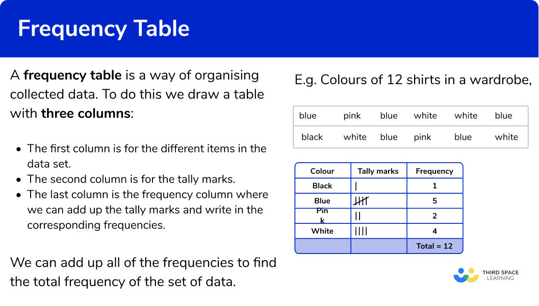
The process of building a frequency table differs slightly depending on the type of data you're working with, a concept we've discussed in previous lessons.
Creating Frequency Tables for Different Data Types
The resource from "Statistics by Jim" provides an excellent overview of how to approach creating frequency tables for categorical, ordinal, and continuous data.
Frequency Table: How to Make & Examples
This article clearly demonstrates how to build frequency tables based on the type of data, which is a crucial first step in data summarization.
Please read the entire article. Start with the introduction. Then, pay close attention to the three main examples: The categorical data example using pet ownership. The ordinal data example using dining satisfaction ratings. The continuous data example using heights, which introduces the important idea of grouping data.
As you read, note the key difference:
- For categorical and ordinal data, the categories already exist. The main task is to count. For ordinal data, we must maintain the natural order in our table.
- For continuous data (or quantitative data with many unique values), listing every single value would create a table as long as the original dataset! Instead, we group the data into intervals or bins. This process is also known as discretization.
Grouped Frequency Distributions: The Art of Binning
Creating grouped frequency tables is a common task in data analysis. The choice of intervals can significantly affect how the distribution appears, so it's important to follow some established guidelines. This process involves a trade-off: wider intervals create a simpler, more readable table but lose more of the original data's detail. Given your computer science background, you can think of this as a form of lossy compression for data summarization.
The following video provides a concise overview of the rules and considerations for creating grouped frequency tables.
How to Interpret (and Create) Frequency Distribution Tables
This video, "How to Interpret (and Create) Frequency Distribution Tables", explains the rationale behind grouping data and the best practices for creating class intervals.
Please watch the segment from the beginning of this section. Focus on the key guidelines for choosing class intervals: Aiming for an appropriate number of rows (5-15 is a good rule of thumb). Choosing simple, whole numbers for interval widths (e.g., 2, 5, 10). Ensuring the bottom value of each interval is a multiple of the interval width. Making sure there are no gaps or overlaps.
The LibreTexts resource provides a more detailed, mathematical approach to constructing these intervals.
2.4: Frequency Distribution Tables - Statistics LibreTexts
This resource offers a formal set of rules for constructing intervals and highlights the importance of including rows with zero frequency to avoid misinterpretation.
Read the section Creating Frequency Distributions using Intervals. Pay attention to the systematic process of determining interval size based on the data's range. Then, read the section Retaining Empty Rows, which explains a crucial point about proper table construction.
A Practical Walkthrough: Building a Complete Table
Now that we have the theory, let's walk through the construction of a complete frequency table step-by-step. A standard frequency table often includes more than just the frequency counts. We can add columns for relative frequency and cumulative frequency to gain even more insight.
- Relative Frequency: The frequency of a category divided by the total number of observations. It is usually expressed as a percentage and tells us the proportion of the data that falls into each category.
- Cumulative Frequency: The running total of the frequencies as you move down the table. The last entry in this column is always the total sample size.
The following video from the "Math and Science" channel provides an excellent, detailed walkthrough of building a table from raw data and then using it to answer questions.
Understand Frequency Tables, Cumulative & Relative Frequency in Statistics - [7-7-3]
This video, "Understand Frequency Tables, Cumulative & Relative Frequency in Statistics", does a fantastic job of taking you from a messy list of numbers to a powerful summary table, explaining each column's purpose along the way.
We will watch this video in parts to break down the process: Constructing the Frequency Column: Watch from the beginning to this point. The instructor takes raw data about thermostat settings, identifies the unique values, and counts their frequencies. Adding the Cumulative Frequency Column: Continue watching from this segment to see how to calculate the running total. Adding the Relative Frequency Column: Now watch this section where the instructor calculates the percentage for each category. This is often the most useful column for interpretation. Interpreting the Final Table: Finally, watch from this part to see how the completed table makes it easy to answer questions about the data, such as "what percentage of people prefer a setting above 71 degrees?" You can then optionally watch the second example (favorite colors) to see the same principles applied to categorical data.
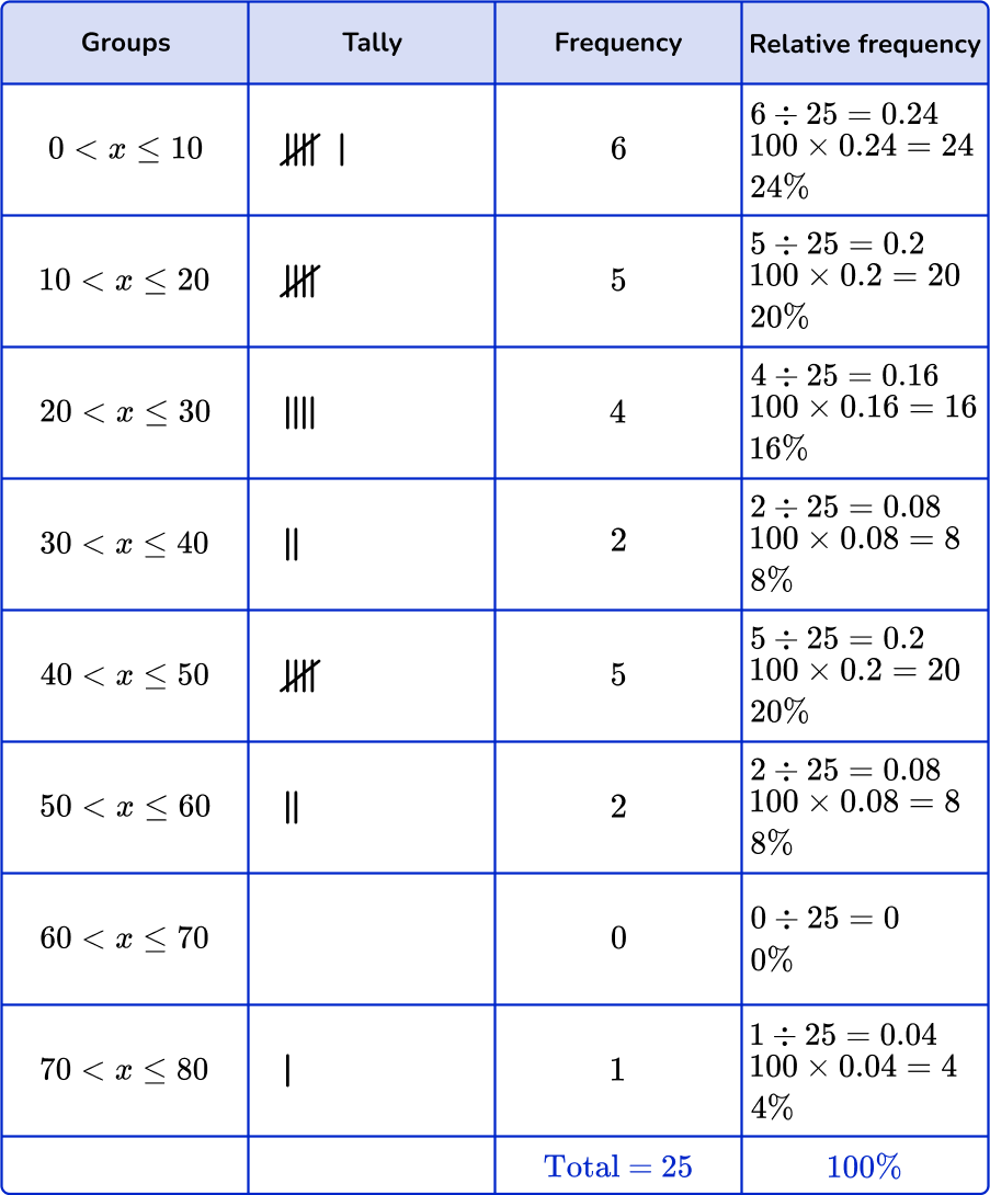
Here is an example of a completed grouped frequency table, similar to the ones you've just learned to construct. It includes groups, tallies, frequencies, and the calculated relative frequencies.
Conclusion
In this lesson, we took our first step into Exploratory Data Analysis by learning how to organize raw data into frequency distribution tables. This foundational skill allows us to condense large, chaotic datasets into structured, interpretable summaries.
Key Takeaways:
- A frequency table summarizes a dataset by showing how often each value or category occurs (its frequency).
- For categorical and discrete quantitative data with few unique values, we create an ungrouped table by listing each unique value.
- For continuous quantitative data or data with many unique values, we create a grouped table by binning values into mutually exclusive, equal-width intervals.
- Relative frequency (proportion/percentage) and cumulative frequency (running total) are additional columns that provide deeper insights into the distribution of the data.
You have now learned how to summarize a distribution in a table. In our next lesson, we will learn how to visualize these same distributions by creating bar charts and histograms, which are essentially graphical representations of the frequency tables you've just mastered.