Hello!
In our last lesson, we learned how to distill raw data into organized frequency distribution tables. This was our first step in Exploratory Data Analysis (EDA), turning a jumble of numbers into a structured summary. While tables are precise, they aren't always the quickest way to grasp the 'story' in the data. Our brains are wired to process visual information rapidly.
This lesson builds directly on our previous work. We will take the information from those frequency tables and learn how to represent it graphically. By the end of this session, you will be able to create and interpret bar charts for categorical data and histograms for quantitative data, two of the most fundamental and widely used tools in a statistician's toolkit. Understanding when and how to use each is crucial for accurately presenting data.
Bar Charts: Visualizing Categorical Data
Let's begin with the simpler of the two plots. A bar chart is used to display the frequencies of categorical data. The process is straightforward: each category gets its own bar, and the height of that bar is proportional to the frequency of that category.
Think back to the frequency table for 'favorite colors' or 'pet ownership' from our last lesson. A bar chart is simply a visual representation of that table.
The resource "Types of Data and Appropriate Representations" from Numeracy Pressbooks provides a good formal introduction. It correctly links data types, which we've covered before, to their appropriate visualizations.
4-3: Types of Data and Appropriate Representations – Numeracy
This text explicitly connects the types of data we've studied (nominal, ordinal) to the use of bar charts and provides a clear example.
First, read the brief section on Ordinal Data, which establishes the connection between categorical data and bar graphs. Next, scroll down to the "Types of Graphs and Charts" section and read the paragraph defining bar graphs. Then, examine the example provided in "Explore 3 – Bar Graphs" and its accompanying interpretation questions. You can find this material by searching for the heading "Explore 3 – Bar Graphs".
As you read, focus on two key characteristics of bar charts:
- Gaps Between Bars: The bars are separated by spaces. This visually reinforces the fact that the categories are distinct and separate entities (e.g., 'cat', 'dog', 'fish' are not points on a continuous scale).
- Order of Bars: For nominal data (like 'country of origin'), the bars can be reordered. It is often helpful to sort them by height to quickly see the most and least common categories. For ordinal data (like 'satisfaction rating'), you must preserve the natural order of the categories.
A bar chart's primary purpose is to allow for the quick comparison of quantities across different groups.
Histograms: Visualizing Quantitative Data
While bar charts handle categories, histograms are used to visualize the distribution of quantitative data (either discrete or continuous). This is where the grouped frequency tables we created in the last lesson become essential. A histogram is the graphical equivalent of a grouped frequency table.
The concept can be subtle, so let's start with a highly intuitive explanation from StatQuest.
StatQuest: Histograms, Clearly Explained
This video brilliantly explains why we need histograms when dealing with many quantitative measurements.
Watch from the beginning to this timestamp. Pay close attention to how the video moves from a messy collection of data points to grouping them into "bins" to create a meaningful shape.
As the video showed, a histogram works by:
- Dividing the entire range of the data into a series of equal, adjacent intervals, called bins.
- Counting how many data points fall into each bin.
- Drawing a bar for each bin, where the height of the bar represents the frequency (the count of data points in that bin).
This image illustrates the process perfectly, taking a raw dataset of ages and transforming it into a histogram.
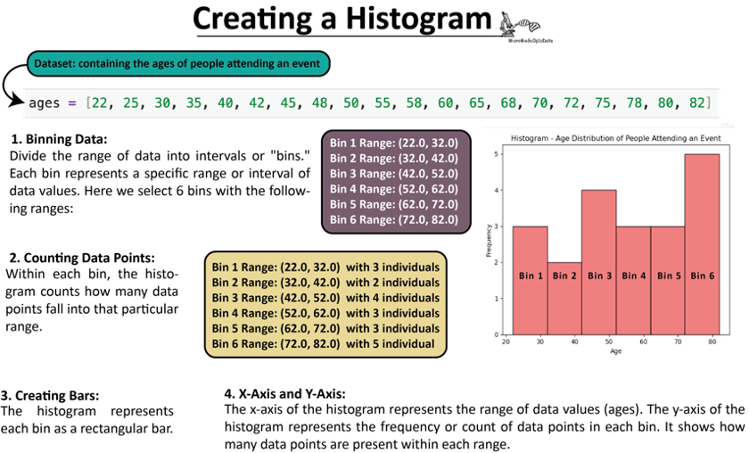
Unlike a bar chart, the bars in a histogram touch each other. This signifies that the x-axis represents a continuous numerical scale, and the bins are adjacent intervals along that scale. Because the x-axis has a fixed numerical order, you cannot reorder the bars of a histogram.
The Critical Distinction: Bar Chart vs. Histogram
Confusing bar charts and histograms is a common mistake, but one that has significant consequences for data interpretation. The choice is not aesthetic; it is dictated entirely by the type of data you are visualizing.
This image provides an excellent side-by-side comparison of their defining features.
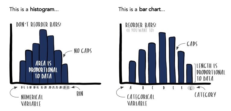
To solidify this distinction, let's consult the "Numeracy" resource again, which explicitly lists the differences.
4-3: Types of Data and Appropriate Representations – Numeracy
This resource provides a concise, text-based explanation of the differences, reinforcing the visual summary above.
Please locate the section titled "Histograms" (you can search for this heading). Read the paragraphs explaining what a histogram is and how it differs from a bar chart. Then, scroll down past the "Example" section and read the three bullet points that directly answer the question, "Name three (3) differences...".
A Practical Challenge: The Bin Width Problem
With bar charts, the categories are predefined. With histograms, you must define the bins. The number (and therefore, width) of these bins can dramatically alter the appearance and interpretation of the histogram.
Given your computer science background, you can think of the bin width as a crucial parameter for your visualization algorithm. Choosing the right value is key to getting a useful output.
- Too many narrow bins: The histogram becomes overly detailed and noisy, showing every minor fluctuation. It's like looking at an image that's all pixels and no clear picture.
- Too few wide bins: The histogram becomes over-simplified, hiding important features of the distribution's shape. It's like looking at a heavily pixelated, low-resolution image.
The StatQuest video you watched earlier has an excellent segment on this exact problem.
StatQuest: Histograms, Clearly Explained
This final segment demonstrates the practical importance of experimenting with bin width to find the most informative visualization.
Please re-watch the section from this timestamp. Notice how the same underlying data can tell very different stories depending on how it's binned.
There are formal rules for choosing an optimal bin width (like Sturges' Rule or the Freedman-Diaconis Rule), but a common practice in EDA is to simply try a few different widths until the key features of the data's distribution become clear.
Conclusion
In this lesson, we transitioned from summarizing data in tables to visualizing it with graphs. We established the clear distinction between bar charts and histograms, a fundamental concept in data presentation.
Key Takeaways:
- Bar charts are used for categorical data. They have gaps between the bars, and for nominal data, the bars can be reordered for easier comparison.
- Histograms are used for quantitative data. Their adjacent bars represent contiguous intervals (bins) on a numerical scale and cannot be reordered.
- The primary purpose of a bar chart is to compare counts between distinct categories. The primary purpose of a histogram is to reveal the underlying frequency distribution of a dataset.
- For histograms, the choice of bin width is a critical parameter that can significantly affect the graph's interpretation.
You now know how to visualize the frequency of single variables. Our next lesson will introduce another powerful visualization, the boxplot. We'll see how it uses the five-number summary (which relies on the quartiles you've already learned to calculate) to provide a compact yet comprehensive view of a variable's distribution and help us identify potential outliers.