Welcome to the next lesson in our exploration of data visualization. In our previous session, we saw how bar charts and histograms can turn raw frequency counts into intuitive graphs that reveal the underlying distribution of a variable. Histograms, in particular, give us a detailed look at the shape of quantitative data.
Today, we will learn how to construct and interpret a boxplot using the five-number summary. A boxplot, also known as a box-and-whisker plot, offers a different but equally powerful way to visualize a distribution. Instead of showing the frequency of every bin like a histogram, a boxplot provides a concise summary, highlighting a dataset's center, spread, and skewness, all in one compact graphic. This makes it an invaluable tool for Exploratory Data Analysis (EDA), especially when comparing multiple groups side-by-side.
The Anatomy of a Boxplot
At its heart, a boxplot is a visual representation of the five-number summary, a concept that brings together several measures we've already studied:
- Minimum: The smallest value in the dataset.
- First Quartile (Q1): The 25th percentile.
- Median (Q2): The middle value of the dataset (the 50th percentile).
- Third Quartile (Q3): The 75th percentile.
- Maximum: The largest value in the dataset.
These five numbers divide the data into four sections, each containing approximately 25% of the data points. The image below illustrates how these five summary statistics are mapped onto the visual components of the plot.
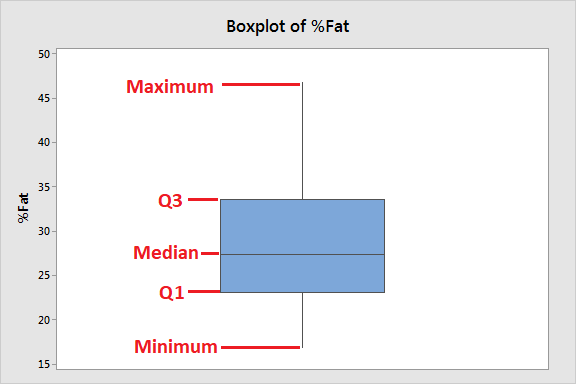
The central "box" is particularly important. It spans from Q1 to Q3, and its length represents the Interquartile Range (IQR), which we know is calculated as . This box contains the middle 50% of the data, providing a robust measure of the data's spread that isn't affected by extreme values.
Let's get a formal overview of these components from the "Box Plot Explained" article by Statistics By Jim.
Box Plot Explained with Examples
This resource clearly outlines the components of a boxplot and connects them to the five-number summary.
Please read the section titled "Anatomy of a Box and Whisker Plot." Pay close attention to the diagrams that show how the five numbers form the plot and how a boxplot relates to a probability distribution function.
Constructing a Boxplot: An Algorithmic Approach
Building a boxplot is a systematic process. Given your computer science background, you can think of it as an algorithm that takes a list of numbers as input and produces a standardized visualization. The most common type of boxplot, and the one we will focus on, is the "modified" boxplot, which explicitly identifies outliers.
The steps are as follows:
- Order the Data: Arrange your dataset in ascending order.
- Calculate Quartiles: Find the median (Q2), the first quartile (Q1), and the third quartile (Q3).
- Calculate the IQR: Compute the interquartile range: .
- Identify Outlier Fences: Calculate the lower and upper limits (often called "fences") beyond which any data point is considered an outlier.
- Lower Fence =
- Upper Fence =
- Determine Whisker Endpoints:
- The lower whisker extends to the smallest data point that is within the lower fence.
- The upper whisker extends to the largest data point that is within the upper fence.
- Draw the Plot:
- Draw a box from Q1 to Q3.
- Draw a line inside the box at the median (Q2).
- Draw the whiskers from the box to the whisker endpoints identified in step 5.
- Plot any data points that fall outside the fences as individual points (dots, asterisks, etc.). These are your outliers.
Watching a worked example is the best way to see this algorithm in action. The following video walks through the entire process for two different datasets, one without outliers and one with.
How To Make Box and Whisker Plots
This video provides a clear, step-by-step demonstration of the boxplot construction algorithm, including the crucial outlier detection step.
First, watch the example without outliers. This will solidify the core process of finding the quartiles and drawing the basic structure. Next, watch the second example with an outlier. Pay close attention to how the 1.5 * IQR rule is used to identify the outlier and how this changes the endpoint of the upper whisker.
To complement the video, here is a textual resource from GeeksforGeeks that also provides a step-by-step calculation. It's a great quick reference for the formulas and the process.
This article concisely explains the IQR rule for outliers and provides another clear, numerical example of the construction process.
First, read the two subsections under "Interquartile Range (IQR)": the definition of IQR and the formulas for identifying outliers. Then, carefully follow the worked example under the heading "How to Create a Box Plot." This walks through the same five steps we outlined above.
Interpreting a Boxplot: Reading the Story
Now that we know how to build a boxplot, let's focus on what it tells us. A boxplot's power lies in its ability to summarize key characteristics of a distribution at a glance.
1. Central Tendency
The median line shows the center of the data. When comparing multiple boxplots, you can quickly see which group has a higher or lower central value by comparing the positions of their medians.
2. Dispersion or Spread
The spread of the data can be assessed in two ways:
- The Interquartile Range (IQR): The length of the box () shows the spread of the middle 50% of the data. A longer box means higher variability.
- The Overall Range: The distance between the ends of the whiskers shows the range of the bulk of the data (excluding outliers). Longer whiskers also indicate greater spread.
3. Skewness
The symmetry of the data is revealed by the position of the median line within the box and the relative lengths of the two whiskers.
- Symmetrical Distribution: The median is roughly in the center of the box, and the whiskers are approximately equal in length.
- Right (Positive) Skew: The median is closer to the bottom (Q1) of the box, and the upper whisker is longer than the lower whisker. This indicates a "tail" of high-value data points.
- Left (Negative) Skew: The median is closer to the top (Q3) of the box, and the lower whisker is longer than the upper whisker. This indicates a "tail" of low-value data points.
The "Statistics by Jim" article provides excellent visual examples for each of these interpretive points.
Box Plot Explained with Examples
This reading will help you learn how to extract meaning from the visual features of a boxplot.
Please read the section titled "How to Read a Box Plot" to see how to assess central tendency, variability, and skewness. Then, look at the final example to see these concepts applied to compare four different groups.
By mastering these three aspects—center, spread, and shape—you can use boxplots to quickly compare distributions, a task that is fundamental to data analysis and a precursor to many statistical tests.
Conclusion
In this lesson, we delved into one of the most efficient visualizations in statistics: the boxplot. We've seen that it's more than just a simple chart; it's a dense summary of a dataset's key distributional characteristics.
Key Takeaways:
- A boxplot is a graphical representation of the five-number summary: minimum, Q1, median, Q3, and maximum.
- The construction of a modern boxplot follows a clear algorithm that uses the 1.5 * IQR rule to establish "fences," which define the ends of the whiskers and identify potential outliers.
- Interpreting a boxplot allows for a quick assessment of a distribution's central tendency (median), spread (IQR and whisker range), and skewness (asymmetry of the box and whiskers).
- Boxplots are particularly powerful for comparing distributions across different categories or groups in a compact and visually effective manner.
We have now laid the groundwork for using boxplots as an analytical tool. In the next lesson, we will focus specifically on that last point: using the IQR method and boxplots to formally identify and analyze potential outliers, a critical step in data cleaning and preparation for modeling.