Welcome to the next lesson in our journey through descriptive statistics. In the last few sessions, we've focused on summarizing a dataset as a whole, first by finding its center (mean, median, mode) and then by measuring its overall spread (standard deviation, coefficient of variation). Now, we will shift our perspective slightly. Instead of looking at the entire dataset at once, we'll learn how to pinpoint the location of values within the dataset.
This lesson introduces quartiles, which are fundamental positional measures. You'll learn how to define and calculate the three quartiles (Q1, Q2, and Q3) that divide a sorted dataset into four equal parts. This skill is not just a calculation exercise; it's the bedrock for understanding a distribution's shape, identifying potential outliers, and constructing one of the most powerful tools in exploratory data analysis: the boxplot.
What Are Quartiles?
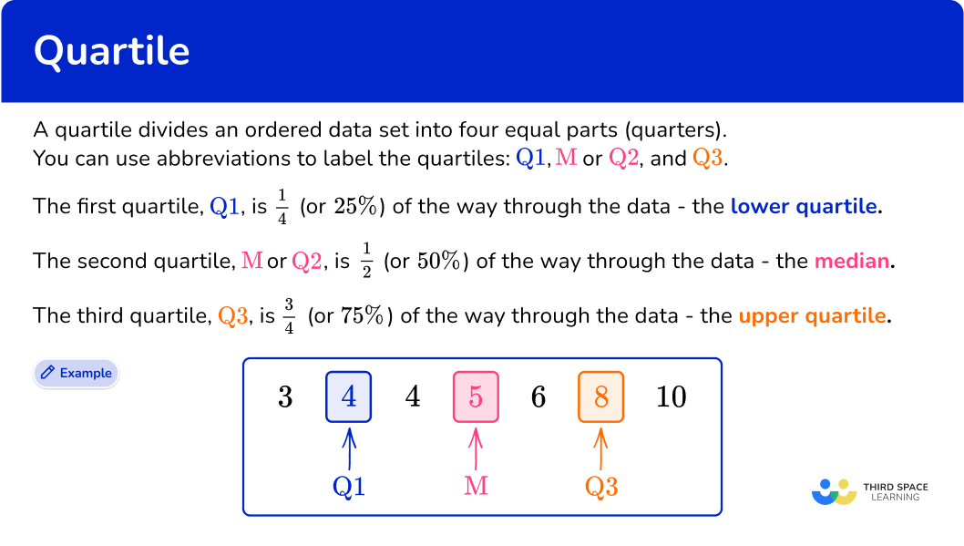
At its core, a quartile is a boundary marker. Imagine you have a set of data—say, the test scores of a class—and you sort them from lowest to highest. The quartiles are the three specific scores that divide this sorted list into four equal-sized groups.
- The First Quartile (Q1) is the value that separates the lowest 25% of the data from the rest. It's also known as the 25th percentile.
- The Second Quartile (Q2) is the value that splits the data in half. 50% of the data is below it, and 50% is above it. As you might have guessed, this is simply the median, a concept we've already covered. It's also the 50th percentile.
- The Third Quartile (Q3) is the value that separates the highest 25% of the data from the rest. 75% of the data lies below it. It's also known as the 75th percentile.
The following images provide a clear visual representation of this concept.

The video below offers a concise animated explanation that links quartiles, percentiles, and the median.
Quartiles, Deciles, & Percentiles With Cumulative Relative Frequency - Data & Statistics
This segment from The Organic Chemistry Tutor provides a great introduction to the relationship between quartiles and percentiles.
Watch the first part of the video, from the beginning up to the explanation of how Q1, Q2, and Q3 correspond to the 25th, 50th, and 75th percentiles. Note the analogy of Q2 being the median of the entire dataset, while Q1 and Q3 are medians of the lower and upper halves.
Calculating Quartiles: The Median-of-Halves Method
Given your background in computer science, you can think of calculating quartiles as a recursive process. The most intuitive method involves repeatedly finding the median.
Here is the step-by-step procedure:
- Order the data: Arrange your dataset in ascending order.
- Find the Second Quartile (Q2): Calculate the median of the entire dataset. This value is Q2.
- Divide the data: The median (Q2) splits the data into a lower half and an upper half.
- If the number of data points (
n) is odd, the median is a single value in the dataset. Exclude this value when forming the lower and upper halves. - If
nis even, the median is the average of the two middle values. The dataset splits perfectly into a lower half and an upper half.
- If the number of data points (
- Find the First Quartile (Q1): Calculate the median of the lower half of the data. This value is Q1.
- Find the Third Quartile (Q3): Calculate the median of the upper half of the data. This value is Q3.
This method is straightforward and builds directly on the concept of the median, which you already know. The following video demonstrates this process for both odd and even sized datasets.
Quartiles, Deciles, & Percentiles With Cumulative Relative Frequency - Data & Statistics
This video by The Organic Chemistry Tutor provides clear, worked examples of the median-of-halves method.
First, watch the example with an odd number of data points from the calculation of quartiles. Observe how the median (Q2) is identified and excluded, and then the medians of the remaining lower and upper halves become Q1 and Q3. Next, watch the example with an even number of data points from this section. Notice how the median (Q2) is the average of the two middle values, and the data splits cleanly into two halves for the calculation of Q1 and Q3.
A Note on Different Calculation Methods
One of the interesting (and sometimes confusing) aspects of statistics is that there isn't always one single, universally-agreed-upon formula for a given measure. This is the case for quartiles. While the median-of-halves method is very common and intuitive, other methods exist. Different software packages (like Excel, Python's pandas library, or R) may use slightly different underlying algorithms, leading to small variations in the calculated quartile values, especially with small datasets.
This is analogous to having different sorting algorithms in computer science (like merge sort vs. quicksort) that achieve the same goal through different procedures. For our purposes, the median-of-halves method is an excellent and reliable approach. However, to give you a sense of the alternatives, let's briefly look at another common technique: the locator method.
8.1 Percentiles and Quartiles – Business/Technical ...
This text from "Business/Technical Mathematics" provides detailed, step-by-step examples of the median-of-halves method, which it calls "Method 1".
First, read through the example under "Method 1" for a dataset with an odd number of values (n=13). This will reinforce the process you saw in the video. Next, scroll down to the next section also titled "Method 1" and read the example for a dataset with an even number of values (n=14). Start from this example to see the procedure applied when the median is not part of the original data.
This resource also describes a "Method 2" that uses formulas to find the position of the quartiles. This is similar to other locator-based methods. You don't need to master it, but it's good to be aware that these formula-based approaches exist and are used in practice. For instance, another popular locator method, demonstrated in the video below, uses the formula L = 0.25 * n to find the position.
Measuring Variation: Quartiles and Five Number Summary
This video from Mathispower4u explains a different "locator method" and provides a full example.
Watch from the explanation of the locator method to understand the rules. Notice how it handles cases where the locator L is a decimal versus a whole number. Then, watch the worked example to see it in action. You might notice the results are slightly different from what the median-of-halves method would produce for the same data. This is perfectly normal and highlights the methodological differences.
For this course, we will primarily rely on the intuitive median-of-halves method. It is easy to compute by hand and conceptually clear. The key is to be consistent in your approach.
Conclusion
In this lesson, we've moved beyond single-point summaries to understand how data is partitioned. Quartiles provide a more nuanced view of a dataset's structure, dividing it into four meaningful chunks.
Key Takeaways:
- Quartiles are positional values that divide a sorted dataset into four equal parts.
- Q1 is the 25th percentile, Q2 is the median (50th percentile), and Q3 is the 75th percentile.
- The most intuitive way to calculate them is the median-of-halves method: find the median of the entire dataset (Q2), then find the medians of the lower and upper halves to get Q1 and Q3.
- Be aware that different calculation methods exist, which may lead to slightly different results. Consistency is key.
These concepts are not just theoretical. In upcoming lessons, we'll see how quartiles are the building blocks for the interquartile range (IQR), a robust measure of spread, and for constructing boxplots, a vital tool for visualizing distributions and identifying outliers. In our very next lesson, we will generalize this idea of dividing data by exploring deciles (dividing data into 10 parts) and percentiles (dividing data into 100 parts).