Measures of Data Spread: Variance and Standard Deviation

From Deviations to Variance

To build a measure of spread that uses all data points, a logical starting point is to consider each point's distance, or deviation, from the mean. However, if we simply sum up all these deviations ($x_i-\bar{x}$), the positive deviations (for points above the mean) and negative deviations (for points below the mean) will always cancel each other out, resulting in a sum of zero. This tells us nothing about the spread.

To solve this, statisticians square each deviation before averaging them. Squaring makes all values positive, so they accumulate rather than cancel. This average of the squared deviations from the mean is called the variance.

The resource below explains this reasoning very clearly.

As you've read, squaring not only solves the zero-sum problem but also gives more weight to larger deviations, a property that is mathematically useful. The squaring operation leads us to the core concept of variance.

Population vs. Sample: The n-1 Enigma

The exact formula for variance depends on whether you have data for the entire population or just a sample.

• Population Variance (${\sigma }^2$): If you have data for every member of a population (a rare scenario), you calculate the variance by taking the average of the squared deviations from the population mean ($\mu$), dividing by the total number of data points, $N$.
  ${\sigma }^2=\frac{{\sum }_{i=1}^N(x_i-\mu {)}^2}{N}$

• Sample Variance ($s^2$): More commonly, we work with a sample to estimate the population variance. Here, we use the sample mean ($\bar{x}$) and divide by $n-1$, where $n$ is the sample size.
  $s^2=\frac{{\sum }_{i=1}^n(x_i-\bar{x}{)}^2}{n-1}$

Why divide by $n-1$ and not $n$? This is a crucial point in statistics. The sample mean, $\bar{x}$, is calculated from the sample itself. By its nature, it is the value that minimizes the sum of squared deviations for that specific sample. This means the deviations from the sample mean tend to be smaller than the deviations from the true (and unknown) population mean, $\mu$. If we divided by $n$, our estimate of the variance would be systematically too low (a biased estimate).

Dividing by the smaller number $n-1$ (this is called Bessel's correction) inflates the variance estimate just enough to correct for this underestimation, giving us a more accurate, or unbiased, estimate of the true population variance.

The following videos provide excellent intuition for this concept, which is often termed "degrees of freedom."

Standard Deviation: Making Variance Interpretable

While variance is a powerful mathematical tool, its units are squared (e.g., dollars-squared, meters-squared), which makes direct interpretation difficult. The solution is simple: we take the square root of the variance to get the standard deviation.

The standard deviation returns the measure of spread to the original units of the data, making it far more intuitive. It represents a "typical" or "standard" distance of a data point from the mean.

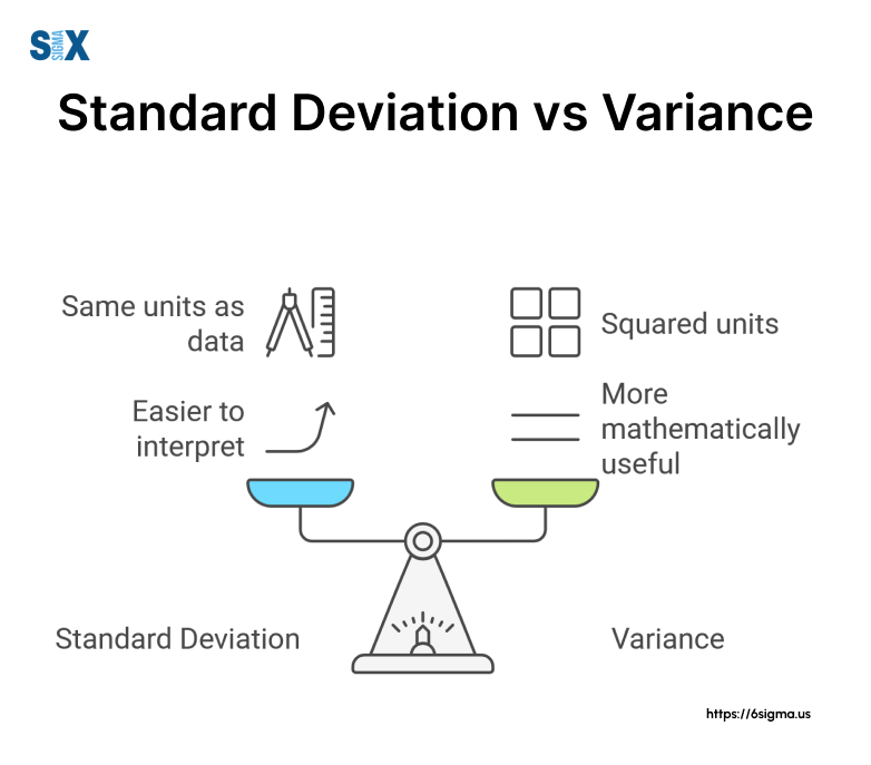
The article from JMP explains this relationship well.

Calculation in Practice

Let's put this all together. Since we almost always work with samples in data science, we will focus on the sample standard deviation ($s$).

The steps to calculate the sample standard deviation are algorithmic:

1. Calculate the sample mean ($\bar{x}$).
2. For each data point $x_i$, calculate its deviation from the mean ($x_i-\bar{x}$).
3. Square each of these deviations.
4. Sum all the squared deviations.
5. Divide the sum by $n-1$ to get the sample variance ($s^2$).
6. Take the square root of the variance to get the sample standard deviation ($s$).

Let's walk through an example.

Interpreting Standard Deviation

The final, and most important, step is interpretation. A standard deviation value tells you how tightly the data are clustered around the mean.

• A low standard deviation indicates that the data points tend to be very close to the mean. The data is consistent and has low variability.
• A high standard deviation indicates that the data points are spread out over a wider range of values. The data is less consistent and has high variability.

Just as with the range, the standard deviation is also sensitive to outliers, though less extremely so, because the outlier's large deviation gets squared.

The image Calculating Standard Deviation also shows a "Normal Distribution Curve" with percentages (68%, 95%, 99.7%). This is a preview of a powerful concept called the Empirical Rule, which we will study later. It states that for many bell-shaped datasets, a predictable percentage of data falls within one, two, or three standard deviations of the mean. This demonstrates just how useful the standard deviation is for understanding a distribution's shape and for making statistical inferences.

Conclusion

In this lesson, we moved beyond the simple range to two of the most important measures of dispersion: variance and standard deviation. You now have a robust method for quantifying and interpreting the spread of your data.

Key Takeaways:

• Variance is the average of the squared deviations from the mean. It uses all data points but results in squared units.
• Standard Deviation is the square root of the variance. It is the most common measure of spread because its units match the original data, making it highly interpretable.
• When calculating variance or standard deviation from a sample (which is almost always the case), we divide by $n-1$, not $n$. This provides an unbiased estimate of the true population parameter.
• A smaller standard deviation means data is tightly clustered around the mean; a larger one means it is more spread out.

While standard deviation is a fantastic measure of spread, how do we use it to compare the variability of two datasets that have very different scales or units (e.g., comparing the variability of house prices in dollars to the variability of their sizes in square feet)? This is where standard deviation alone falls short. In our next lesson, we will introduce the coefficient of variation, a measure that solves exactly this problem.