Welcome to the next lesson in our journey through descriptive statistics. In our previous session, we focused on measures of central tendency—mean, median, and mode—and how to choose the right one to describe the "center" of a dataset. However, knowing the center is only half the story. Two datasets can share the exact same mean yet look completely different.
This lesson introduces the other half of the story: variability, or how spread out the data points are. We will start with the simplest measure of dispersion: the range. Your goal for this lesson is to learn how to calculate the range and, more importantly, how to interpret what it tells you about your data, including its significant limitations. This concept is the first step toward quantifying the consistency and spread of data, a fundamental task in any data analysis workflow.
Why Do We Need to Measure Spread?
Imagine you are analyzing the daily server response times for two different cloud providers. Both report an average (mean) response time of 50 milliseconds. Based on this measure of central tendency alone, they appear identical.
However, a closer look reveals:
- Provider A: Response times are tightly clustered, ranging from 45ms to 55ms.
- Provider B: Response times are widely spread, ranging from 10ms to 90ms.
Clearly, Provider A is far more consistent and reliable, even though the average is the same. Measures of central tendency failed to capture this crucial difference in performance. This is why we need measures of dispersion. They quantify the spread of data, providing a more complete picture.
The video below offers a great motivation for why we need measures of variability like the range.
Measures of Variability (Range, Standard Deviation, Variance)
This video from Daniel Storage uses clear, practical examples to illustrate why measures of central tendency alone are insufficient.
Watch the introductory segment from the beginning until the three measures are listed. Pay attention to the two examples—the clustered vs. spread-out scores and the medication effectiveness—to solidify your intuition about the importance of variability.
Calculating the Range
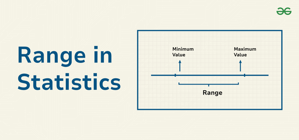
The range is the most straightforward measure of variability. It is simply the difference between the maximum and minimum values in a dataset.
The formula is as simple as it sounds:
Let's use a resource from Statistics by Jim to see a formal definition and a simple calculation.
Range of a Data Set - Statistics By Jim
This article provides a concise definition, the formula, and a clear example of calculating the range.
Read the introduction and the first two sections, "Formula" and "Example of Finding the Range." Focus on understanding the definition and the direct application of the formula to the two sample datasets provided.
As the article demonstrates, if Dataset 1 has a maximum of 38 and a minimum of 20, its range is . If Dataset 2 has a range of 41, we can interpret that Dataset 2 has greater variability than Dataset 1. The range is expressed in the same units as the original data, which makes it very intuitive.
The Critical Limitations of the Range
While the range is easy to calculate, its simplicity is also its greatest weakness. Because it depends only on the two most extreme values, it has two major limitations that you must always consider.
1. Extreme Sensitivity to Outliers
An outlier, a single atypically high or low value, can drastically distort the range, giving a misleading impression of the data's overall spread.
Let's return to the "Range of a Data Set" article to see a powerful example of this.
Range of a Data Set - Statistics By Jim
This section of the article clearly demonstrates how a single outlier can render the range a misleading statistic.
Now, read the section "Limitations of Using the Range." Focus on the example where a single value is changed. Note how the range for Dataset 1 jumps from 18 to 82, as explained in the text from "Let's return to" this part of the article.
This example is critical. The bulk of the data in the modified Dataset 1 is still tightly clustered between 20 and 34. However, because of one outlier (102), the range suggests it is twice as variable as Dataset 2, which is clearly not a fair representation of the data's structure.
2. Ignoring the Data's Distribution
The second limitation follows from the first: the range tells you nothing about how the data points are distributed between the two extremes. Two datasets can have the same range but vastly different internal structures.
The following resource from a STAT 350 course page provides a perfect illustration of this problem.
3.3. Measures of Variability - Range, Variance, and Standard Deviation — STAT 350
This resource shows visually why the range can be a poor measure of spread by comparing three datasets with identical ranges but different distributions.
Read the subsection "Limitations of Sample Range." Pay close attention to the table and the corresponding dot plot showing three datasets that all share the same range but are clearly distributed differently. The text explains this limitation from this point.
As you can see, all three sets have a range of 30, but their shapes are completely different. Set 1 is clustered at the center, Set 3 is concentrated at the extremes, and Set 2 is more uniform. The range fails to capture any of these distinctions. This is because it discards all information except for the two endpoints.
A final, related limitation is that the range tends to increase with sample size. The larger the sample, the more opportunities you have to capture an extreme value. Therefore, comparing the ranges of two datasets of different sizes is often not a meaningful comparison.
When is Range a Useful Measure?
Given these significant limitations, you might wonder if the range is ever useful. It is, but primarily in specific contexts:
- Quick Preliminary Assessment: It gives a very fast, though crude, idea of the data's spread. If you're looking at a new dataset, calculating the range in your head can be a good first step.
- Detecting Data Entry Errors: Its sensitivity to outliers can be turned into a strength. If you are analyzing human height in meters and find a range of 20, you instantly know there's a data entry error.
- Small, Controlled Datasets: For small datasets where you are confident there are no outliers, the range can be a reasonable and simple measure of spread.
Conclusion
In this lesson, you've learned about the most basic measure of variability: the range. You can now calculate it and, more importantly, interpret its meaning and its significant drawbacks.
Key Takeaways:
- Measures of dispersion (or variability) quantify how spread out data points are, providing a necessary complement to measures of central tendency.
- The range is the difference between the maximum and minimum values in a dataset.
- It is simple to calculate and intuitive, as it's expressed in the data's original units.
- Its primary weakness is its high sensitivity to outliers and its complete disregard for the distribution of data between the extremes.
The limitations of the range highlight the need for more robust measures of spread—ones that incorporate every data point into their calculation, not just the two extremes. This is precisely what we will explore in our next lesson, where we will dive into two of the most important concepts in statistics: variance and standard deviation.