Hello! Welcome back to our exploration of Communication Systems.
In our last lesson, we examined the cellular concept, a clever "divide and conquer" strategy that allows a limited set of radio frequencies to serve billions of mobile phones. We saw how systems like your phone manage calls and data on a large, geographical scale.
Today, we're going to zoom in from the network level to the signal level. The previous lesson mentioned that your voice is converted into a digital signal. But what does that actually mean? How can a continuous, flowing sound wave from your voice be transformed into the discrete 1s and 0s that a computer or phone can process?
This brings us to our learning outcome for this lesson: to explain the fundamental idea of analog-to-digital conversion (sampling and quantization). Since you're interested in the deep conceptual underpinnings of technology, this lesson will focus on the "why" and "how" of this crucial process, which forms the bedrock of all modern digital communication.
The Problem: Bridging Two Worlds
The world we experience is fundamentally analog. The sound of a voice, the brightness of light, and the temperature of the air are all signals that vary continuously. They can take on an infinite number of values within a given range.
Computers, however, live in a digital world. They work with discrete, finite information represented as binary digits (bits)—0s and 1s.

To bridge this gap, we need a process called Analog-to-Digital Conversion (ADC). Let's start with a short video that introduces this core distinction.
Converting Analog Data to Binary, Sampling, Quantization - AP Computer Science Principles
The video 'Converting Analog Data to Binary, Sampling, Quantization' by Professor Cunningham clearly explains the difference between the infinite, continuous nature of analog signals and the finite, discrete nature of digital data.
Please watch from 00:22 to 01:16. This will set the stage for why we need to convert from one form to the other.
As the video explains, an analog signal presents two problems for a computer:
- It has infinitely many points in time.
- At any given point, its value (amplitude) has infinite precision.
Analog-to-Digital Conversion solves these two problems with a two-step process: sampling and quantization.
Step 1: Sampling (Making Time Discrete)
The first problem is the infinite number of points along the time axis. We solve this with sampling. Sampling is the process of measuring the amplitude of the analog signal at regular, discrete time intervals. Instead of a continuous line, we now have a sequence of "snapshots."
- The time between two consecutive samples is the sampling interval.
- The number of samples taken per second is the sampling rate (or sampling frequency), measured in Hertz (Hz).
This video segment explains the process visually.
Converting Analog Data to Binary, Sampling, Quantization - AP Computer Science Principles
Let's return to Professor Cunningham's video to see how sampling works and how the sampling rate affects the representation of the original signal.
Watch from 03:00 to 05:25. Focus on how taking samples at regular intervals creates a set of discrete points and how a higher sampling rate (shorter interval) leads to a more faithful representation of the original wave.
The Nyquist-Shannon Sampling Theorem and Aliasing
This raises a critical question: how fast do we need to sample to capture the signal accurately? If we sample too slowly, we might miss important details of the wave, and our digital version will be a poor approximation.
This is answered by one of the most important principles in signal processing: the Nyquist-Shannon Sampling Theorem. It states:
To be able to perfectly reconstruct an analog signal from its samples, the sampling rate () must be at least twice the highest frequency () present in the signal.
The minimum rate, , is called the Nyquist rate.
What happens if we violate this rule and sample too slowly? We get a strange and undesirable effect called aliasing, where a high-frequency signal masquerades as a lower-frequency one in the sampled data.
To build an intuition for this, watch the following video. It demonstrates how sampling a simple 1 Hz sine wave at different rates can create ambiguity.
The intuition behind the Nyquist-Shannon Sampling Theorem
The video 'The intuition behind the Nyquist-Shannon Sampling Theorem' by Zach Star provides a brilliant visual intuition for aliasing without getting into heavy mathematics.
Watch from the beginning to 03:33. Observe what happens when the sampling frequency drops below twice the signal's frequency. You'll see how a completely different, lower-frequency wave can perfectly fit the sampled points.
This is why audio CDs use a sampling rate of 44,100 Hz (44.1 kHz). The range of human hearing tops out at about 20,000 Hz (20 kHz). The CD sampling rate is more than double this highest frequency (), ensuring that all audible frequencies are captured without aliasing.
Step 2: Quantization (Making Amplitude Discrete)
After sampling, we have a series of points that are discrete in time, but their amplitude values are still from the continuous analog world. The second problem is that these values have infinite precision (e.g., 0.70710678... volts). A computer can't store numbers with infinite decimal places.
We solve this with quantization. Quantization is the process of rounding each sample's amplitude to the nearest value on a finite grid of discrete levels.
- The resolution, or bit depth, determines the number of levels. An n-bit converter has distinct levels. For example, a 3-bit converter has levels, while a 16-bit converter has levels.
- The difference between the actual analog sample value and the rounded quantized value is called quantization error. Higher resolution (more bits) means smaller steps between levels and therefore less error.
This next video segment explains quantization clearly.
Converting Analog Data to Binary, Sampling, Quantization - AP Computer Science Principles
Let's watch the final explanatory part of Professor Cunningham's video to understand quantization.
Watch from 07:17 to 09:55. Focus on how the continuous amplitude of each sample is snapped to the nearest discrete level and how the number of available levels (determined by bit depth) affects accuracy.
To truly appreciate the effect of quantization, it's best to hear it. The following resource provides audio examples of a voice saying "Hello" quantized at different bit depths.
Signals - Quantization and Sampling
This guide from the Makeability Lab at the University of Washington provides an excellent demonstration of quantization's effect on audio quality. While the page includes code, you only need to read the text and, most importantly, listen to the audio clips.
Please read through the section titled 'Quantization'. Start from the beginning of this section and go down to the end of the '2-bit quantization' part. As you go, play the audio files for 16-bit, 8-bit, 6-bit, 4-bit, 3-bit, and 2-bit quantization. Notice how 'quantization noise' (a hissing or grainy sound) becomes more prominent as the bit depth decreases.
As you likely heard, 16-bit and 8-bit audio sound quite clear, but the quality degrades rapidly at lower bit depths. By 3 or 2 bits, the voice is barely intelligible. This demonstrates the impact of quantization error.
The Big Picture: Quality vs. Data Size
We have now solved both problems. Sampling makes the signal discrete in time, and quantization makes it discrete in amplitude. The result is a stream of numbers, each representing a specific amplitude level, which can then be easily encoded into binary 0s and 1s.
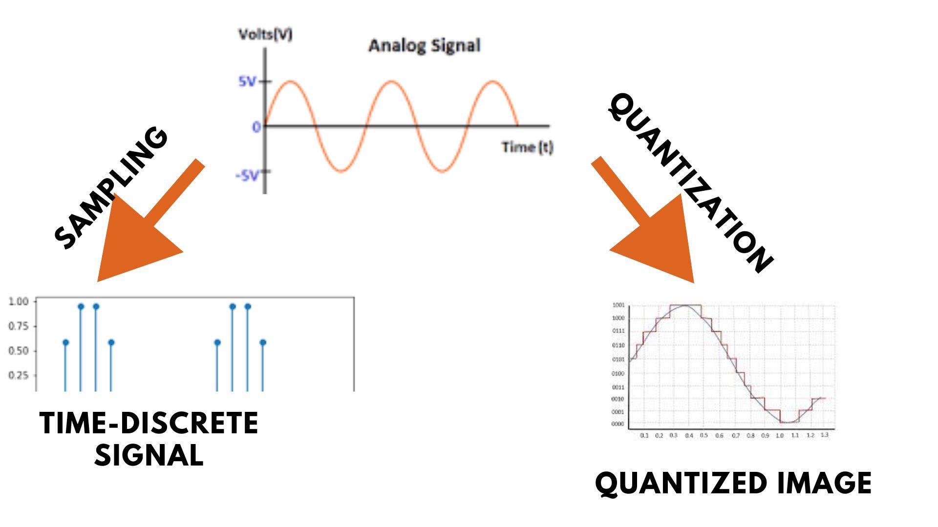
This entire process involves a fundamental trade-off: Quality vs. Data Size.
- Higher Sampling Rate -> More accurate representation of high frequencies, less aliasing -> More data.
- Higher Quantization Resolution (more bits) -> More amplitude levels, less quantization error -> More data.
A high-fidelity music track (like on a CD: 44.1 kHz sampling, 16-bit quantization) sounds fantastic but takes up a lot of space. A telephone call (often 8 kHz sampling, 8-bit quantization) sounds much lower quality but requires far less data, making it efficient for transmission over phone lines. Engineers must always balance the desired quality with the available storage and bandwidth.
Test your understanding!
You are tasked with digitizing two audio signals. Signal A is a recording of a full orchestra for a high-fidelity music album. Signal B is a recording of a person's voice for a simple podcast.
How would you expect the sampling rate and quantization bit depth to be chosen for Signal A versus Signal B? Explain your reasoning based on the concepts of the Nyquist theorem, aliasing, and quantization error.
Show answer
-
Signal A (Orchestra): This signal would require a high sampling rate and a high bit depth.
- Sampling Rate: An orchestra produces a wide range of frequencies, from the low rumbles of a double bass to the high-pitched notes of a piccolo, potentially reaching the limits of human hearing (~20 kHz). According to the Nyquist theorem, to avoid aliasing and capture these high frequencies faithfully, the sampling rate must be high (e.g., 44.1 kHz or higher).
- Bit Depth: The dynamic range (the difference between the quietest and loudest sounds) is very large in an orchestra. A high bit depth (e.g., 16-bit or 24-bit) is needed to provide enough quantization levels to represent both the softest and loudest passages with minimal quantization error, preserving the music's detail and clarity.
-
Signal B (Podcast): This signal can be digitized effectively with a lower sampling rate and a lower bit depth compared to the orchestra.
- Sampling Rate: The human voice has a much more limited frequency range than a full orchestra, with most important frequencies falling below 4 kHz. Therefore, a lower sampling rate (e.g., 8 kHz or 16 kHz) is sufficient to capture the voice intelligibly without significant aliasing of essential frequencies.
- Bit Depth: The dynamic range of a single speaking voice is much smaller than an orchestra's. A lower bit depth (e.g., 8-bit or 12-bit) can provide adequate quality without introducing obvious quantization noise, making the file size smaller and easier to stream.
In short, you tailor the ADC parameters to the characteristics of the signal to balance quality and data efficiency.
Conclusion
In this lesson, we've demystified the process of converting the analog world into the digital language of computers. This is a fundamental concept that enables everything from streaming music and making phone calls to digital photography and medical imaging.
Key Takeaways:
- Analog-to-Digital Conversion (ADC) bridges the gap between continuous real-world signals and discrete digital data.
- The process involves two main steps:
- Sampling: Capturing the signal's amplitude at regular time intervals. The Nyquist-Shannon theorem dictates that the sampling rate must be at least twice the signal's highest frequency to avoid aliasing.
- Quantization: Approximating the amplitude of each sample to one of a finite number of levels, determined by the bit depth. This introduces quantization error.
- There is a direct trade-off between the quality of the digital signal (higher sampling rate and bit depth) and the amount of data it generates.
Preview of the Next Lesson:
Now that we understand how we can represent any signal as a stream of 1s and 0s, the next logical question is: how do we ensure that this stream of bits gets from one place to another (e.g., from a web server to your computer) accurately and reliably, especially across a complex and sometimes unreliable network like the internet? This leads us to our next topic: the role of protocols in ensuring reliable communication.