Introduction
Hello and welcome back!
In our previous lesson, we took a trained logistic regression model and used the Score tool to generate survival probabilities for each passenger in our test dataset. This gave us a nuanced prediction for each individual, but it also left us with a key question: how good are these predictions, really?
Today, we'll answer that question. Our goal is to evaluate model performance using a confusion matrix and related metrics like accuracy, precision, and recall. We will learn how to turn probabilities into concrete predictions and then measure how well those predictions align with reality. This is a critical step in any predictive modeling project and a core competency tested for the Alteryx Advanced Certification.
From Probability to Classification
The Score tool gave us probabilities, such as a 0.78 chance of survival for a given passenger. To evaluate the model, we first need to convert this probability into a definitive classification: "Survived" (1) or "Did not survive" (0).
We do this by setting a cutoff threshold. The most common starting point is 0.5.
- If the probability of survival is > 0.5, we predict "Survived".
- If the probability of survival is <= 0.5, we predict "Did not survive".
In your Alteryx workflow, you can easily create these classifications using a Formula tool after the Score tool. If your Score tool created a field named Survival_Prob_1, the expression would be:
IF [Survival_Prob_1] > 0.5 THEN 1 ELSE 0 ENDIF
This gives you a new column of final predictions that you can compare directly against the actual Survived column in your testing data.
The Confusion Matrix: Comparing Predictions to Reality
Once we have our final predictions, the first step in evaluation is to organize the results in a confusion matrix. This is a simple but powerful table that breaks down a model's performance by comparing its predictions to the actual, true values.
A confusion matrix has four key components:
- True Positive (TP): The model correctly predicted the positive class. (e.g., Predicted 'Survived', and the person actually 'Survived').
- True Negative (TN): The model correctly predicted the negative class. (e.g., Predicted 'Did not survive', and the person actually 'Did not survive').
- False Positive (FP): The model incorrectly predicted the positive class. This is a Type I error. (e.g., Predicted 'Survived', but the person 'Did not survive').
- False Negative (FN): The model incorrectly predicted the negative class. This is a Type II error. (e.g., Predicted 'Did not survive', but the person actually 'Survived').
This video provides a great visual introduction to these concepts.
TP, FP, TN, FN, Accuracy, Precision, Recall, F1-Score, Sensitivity, Specificity, ROC, AUC
To start, let's watch a brief explanation of the four outcomes that form the confusion matrix.
Watch the video from the beginning until timestamp 03:23. Focus on understanding the definitions of True Positive, False Positive, False Negative, and True Negative in the context of the medical diagnosis example.
This structure allows us to move beyond a simple "percent correct" and analyze the types of errors our model is making.
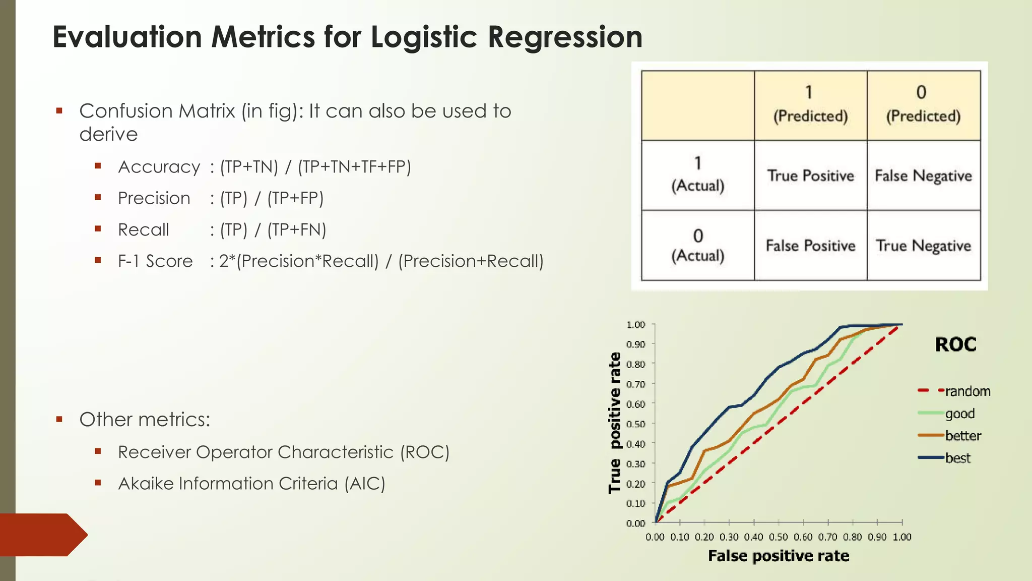
Key Performance Metrics
The confusion matrix provides the raw numbers, but we use several key metrics to summarize model performance.
Metric Matters, Part 1: Evaluating Classification Models
This Alteryx Community article provides clear definitions for the most important classification metrics. We'll use it as a reference as we go through them.
For now, just open this article in another tab. As we define each metric below, refer to the corresponding sections: 'Accuracy', 'Precision', and 'F1 score' (which also defines Recall). Pay attention to the 'Important to know' points, as they explain when each metric is most useful.
1. Accuracy
Accuracy is the most intuitive metric. It answers the question: "Overall, what percentage of predictions did the model get right?"
Formula: (TP + TN) / (TP + TN + FP + FN)
While simple, accuracy can be misleading, especially with imbalanced datasets. If 95% of passengers did not survive, a model that simply predicts "Did not survive" for everyone would be 95% accurate, but it would be completely useless for identifying survivors.
2. Precision
Precision focuses on the positive predictions. It answers the question: "Of all the passengers the model predicted would survive, how many actually did?"
Formula: TP / (TP + FP)
High precision is crucial when the cost of a False Positive is high. For example, in a model that flags emails as spam, you want high precision. You'd rather a few spam emails get through (False Negatives) than have important emails incorrectly sent to the spam folder (False Positives).
3. Recall (or Sensitivity)
Recall also focuses on the positive class but from a different angle. It answers: "Of all the passengers who actually survived, how many did the model correctly identify?"
Formula: TP / (TP + FN)
High recall is vital when the cost of a False Negative is high. In a model for disease detection, you want high recall. You want to find as many actual cases as possible, even if it means some healthy patients are incorrectly flagged for more testing (False Positives).
4. F1-Score
The F1-Score is the harmonic mean of Precision and Recall. It seeks to find a balance between the two. It's particularly useful when you have an imbalanced class distribution.
Formula: 2 * (Precision * Recall) / (Precision + Recall)
An F1-Score punishes models that have an extreme imbalance between precision and recall (e.g., very high precision but very low recall).
To solidify your understanding of these calculations, let's walk through a concrete example.
Confusion Matrix Solved Example Accuracy Precision Recall F1 Score Prevalence by Mahesh Huddar
This video provides a step-by-step solved example of calculating all these metrics from a given confusion matrix.
Watch the following segments to see how each metric is calculated: Definitions (00:44 - 01:39): See how the numbers in the matrix are labeled TP, TN, FP, FN. Accuracy (01:28 - 02:20): Follow the accuracy calculation. Recall (True Positive Rate) (02:40 - 03:27): Follow the recall calculation. Precision (04:13 - 05:08): Follow the precision calculation.
Model Evaluation in Alteryx
While you could build a confusion matrix manually using Formula and Cross Tab tools, Alteryx provides a much more direct way to evaluate your models: the Model Comparison tool.
This tool takes one or more model objects and a test dataset, and it automatically generates a comprehensive report that includes the confusion matrix and all the key metrics we've discussed.
Model Comparison Tool - Alteryx Help
Let's look at the official Alteryx documentation for the Model Comparison tool.
Read the introduction, 'Connect Inputs,' 'Configure the Tool,' and 'View the Output' sections. Pay close attention to: The two required inputs: M (Model) and D (Data). The 'positive class' configuration setting, which is crucial for binary classification. The R (Report) output anchor, which is where we'll find our evaluation metrics.
Your Turn: Evaluate the Titanic Model
It's time to put this into practice. Open the Alteryx workflow you've been building for the Titanic dataset. You should have your data split, a Logistic Regression tool trained on the training data, and a Score tool generating probabilities on the testing data.
- Drag a Model Comparison tool onto your canvas (from the Predictive tool category).
- Connect the 'O' (Object) output anchor of your
Logistic Regressiontool to the 'M' (Model) input anchor of theModel Comparisontool. - Connect your testing data stream to the 'D' (Data) input anchor of the
Model Comparisontool. - In the
Model Comparisontool's configuration, you'll see an option for "The positive class in target variable". Since our goal is to identify survivors, select '1' from the dropdown. This tells Alteryx that '1' (Survived) is the outcome we are focused on for metrics like precision and recall. - Attach a
Browsetool to the 'R' (Report) output anchor of theModel Comparisontool and run the workflow. - Click on the
Browsetool to view the report. You will see a "Type" column for "Overall" and "Class". Look for the Confusion Matrix in the report. Then, find the table of metrics and identify the Accuracy, Precision, Recall, and F1 values for your model.
How did your model do? By analyzing these metrics, you now have a much more sophisticated understanding of your model's performance than a simple accuracy score could ever provide.
Conclusion
Great work today! You've learned how to move from model predictions to a rigorous performance evaluation, which is a cornerstone of applied predictive analytics.
Key Takeaways:
- A cutoff threshold (e.g., 0.5) is used to convert probabilities into firm classifications.
- A confusion matrix is the foundation for evaluation, breaking down predictions into True Positives, True Negatives, False Positives, and False Negatives.
- Accuracy measures overall correctness but can be misleading with imbalanced data.
- Precision and Recall provide a more nuanced view of performance, highlighting the trade-off between different types of errors (False Positives vs. False Negatives).
- The F1-Score provides a balanced measure between precision and recall.
- In Alteryx, the Model Comparison tool automates the calculation of these metrics, providing a detailed performance report.
Preview of the Next Lesson:
The metrics we calculated today were based on a single, fixed cutoff of 0.5. But what if a different cutoff would give us a better balance of precision and recall for our specific business problem? And how does our model's performance compare to just random guessing?
In the next lesson, we will explore tools that evaluate model performance across all possible thresholds. We'll learn how to use the Lift Chart and ROC Curve tools to visualize and compare model performance, giving us an even deeper insight into our model's effectiveness.