Visualizing Model Performance with Lift Charts and ROC Curves

Part 1: The Lift Chart

A lift chart answers a practical business question: "How much better is my model at finding positive outcomes than a random guess?"

Imagine you want to send a marketing offer to customers most likely to respond. You only have the budget to contact 10% of your customer base. A good model should ensure that this 10% contains a much higher concentration of responders than you'd find in a random 10% sample of the population. The lift chart quantifies this "boost."

How it Works:

1. The model scores every record in your test dataset and sorts them from the highest probability of being a "positive" case to the lowest.
2. The sorted data is divided into equal-sized groups, typically ten groups called deciles. The top decile contains the 10% of records the model is most confident about.
3. The chart then plots the "lift" for each decile. Lift is the ratio of positive cases found by the model in that decile versus the number you would expect to find with a random selection.

• A lift of 1.0 means the model is no better than a random guess.
• A lift of 3.0 in the top decile means that by targeting the top 10% of records ranked by the model, you will reach 3 times as many positive cases as you would by targeting a random 10% of the population.

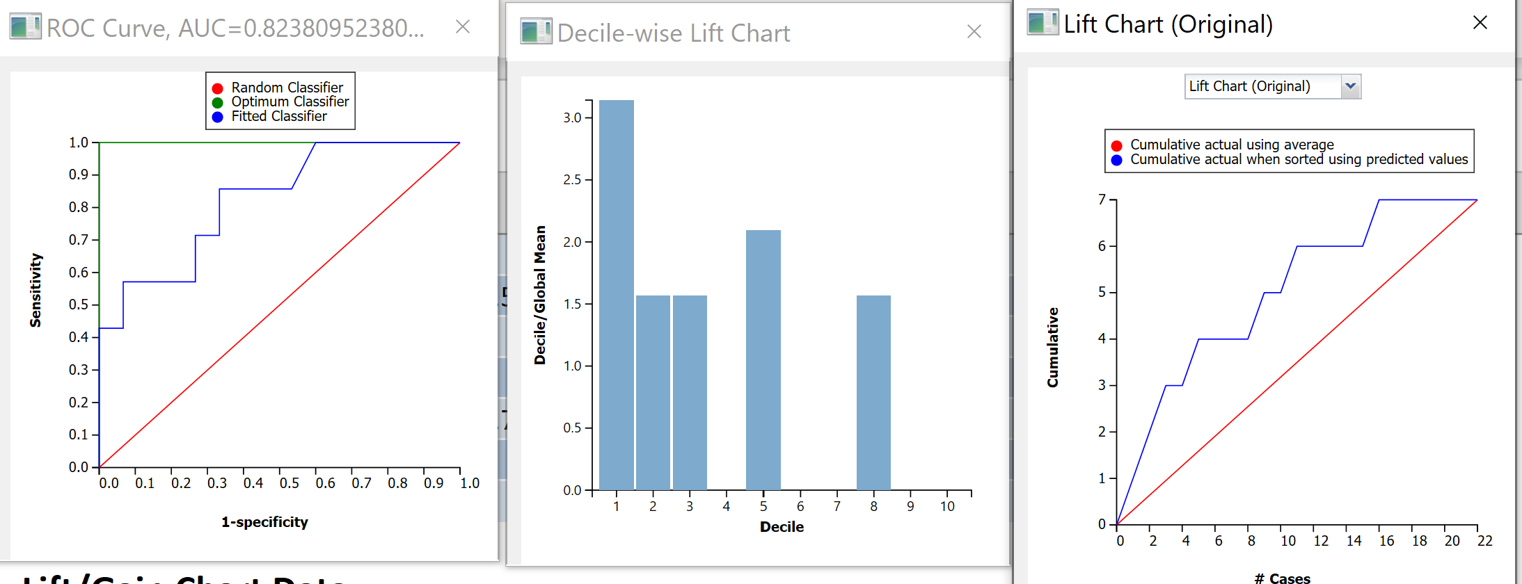
In Alteryx, while there is a dedicated Lift Chart tool, the Model Comparison tool automatically generates these plots for you in its report output (R anchor). This is usually the most efficient way to get them.

Part 2: The ROC Curve and Area Under the Curve (AUC)

The Receiver Operating Characteristic (ROC) curve is one of the most important evaluation tools for a binary classifier. It provides a complete picture of the trade-off between a model's benefits and costs across every possible threshold.

The curve plots two key metrics that you'll recall from our previous lesson:

• Y-axis: True Positive Rate (TPR), also known as Sensitivity or Recall.
  $\text{TPR}=\frac{\text{True Positives}}{\text{True Positives}+\text{False Negatives}}$
  This is the proportion of actual positives the model correctly identifies. You want this to be high.

• X-axis: False Positive Rate (FPR).
  $\text{FPR}=\frac{\text{False Positives}}{\text{False Positives}+\text{True Negatives}}$
  This is the proportion of actual negatives the model incorrectly flags as positive. You want this to be low.

To understand how these two rates create the curve, it's best to see it built step-by-step.

Interpreting an ROC Curve

Now that you've seen how an ROC curve is built, let's learn how to interpret its shape.

As you saw, the key interpretations are:

• Diagonal Line (y=x): Represents a model with no predictive power (random guessing). Any model you build should perform above this line.
• Top-Left Corner (Point [0,1]): Represents a perfect classifier with a 100% True Positive Rate and 0% False Positive Rate.
• The Curve: The closer the curve "bows" toward the top-left corner, the better the model's performance.

Area Under the Curve (AUC)

While the shape of the ROC curve is informative, it's often useful to summarize its performance with a single number: the Area Under the Curve (AUC).

• AUC measures the entire two-dimensional area underneath the ROC curve.
• AUC ranges from 0.5 (for a random model) to 1.0 (for a perfect model).
• A higher AUC represents a better classifier.

AUC has a useful statistical property: it is the probability that the model will rank a randomly chosen positive instance higher than a randomly chosen negative instance. This makes it an excellent metric for comparing different models. If Model A has an AUC of 0.88 and Model B has an AUC of 0.82 on the same test data, you can be confident that Model A is the better-performing model.

Your Turn: Analyze the Titanic Model's Performance

It's time to apply this knowledge. Let's go back to the Alteryx workflow you built for the Titanic dataset, where you used the Model Comparison tool.

1. Run your workflow if you haven't already.
2. Click the Browse tool connected to the R (Report) output of your Model Comparison tool.
3. In the report window, scroll down past the confusion matrix and the metrics table. You will find a section of Performance Diagnostic Plots.
4. Examine the ROC Curve:
   • Find the plot labeled "ROC Curve". You'll see your model's curve (labeled "fitted classifier") and the random guess line.
   • What is the AUC for your model? The value is written directly on the plot.
   • How does your model's curve compare to the random guess line? Is it demonstrating good predictive power?
5. Examine the Lift Chart:
   • Find the plot labeled "Decile-wise Lift Chart".
   • Look at the bar for the first decile (labeled '1' on the x-axis). What is the lift value?
   • In plain English, what does this lift value mean in the context of finding Titanic survivors?

By analyzing these charts, you've now performed a comprehensive evaluation of your classification model, moving beyond a single set of metrics to understand its behavior across the full range of possibilities.

Conclusion

Excellent work today! You have added two of the most powerful and widely-used tools for classifier evaluation to your skillset.

Key Takeaways:

• Metrics like precision and recall depend on a specific classification threshold, which may not be optimal.
• A Lift Chart shows how much more effective your model is at finding positive cases compared to random chance, which is useful for resource allocation problems.
• An ROC Curve visualizes the trade-off between the True Positive Rate and the False Positive Rate across all possible thresholds. The closer the curve is to the top-left corner, the better.
• AUC (Area Under the Curve) provides a single, robust metric for a model's overall performance, making it ideal for comparing different models.
• In Alteryx, the Model Comparison tool is the most direct way to generate reports containing both Lift Charts and ROC curves.

You have now completed the module on classification modeling! You've learned how to build, score, and rigorously evaluate a logistic regression model.

Preview of the Next Lesson:
So far, all our predictive modeling has been a form of supervised learning—we had a known target variable (Survived) that we were trying to predict. In the next module, we will venture into the world of unsupervised learning, where there is no target variable. Our first topic will be explaining the use cases for clustering, a technique used to discover natural groupings and segments in your data, such as customer personas.