Understanding Basic Statistics: Mean, Median, and Standard Deviation

1. Measures of Central Tendency: What is a "Typical" Value?

When you first look at a set of data—like daily sales figures, user session times, or click-through rates on an ad campaign—the first question you'll likely ask is, "What's a typical number here?"

Statisticians call this concept central tendency. It's a way of describing the center of your data with a single, summary value. The three most common measures are the mean, median, and mode.

To get a clear and concise overview of these three measures, let's watch a short video. It uses examples that should be familiar from your AdTech background, such as daily search queries and time spent on an app.

As the video explained, each measure tells a slightly different story:

• Mean (Average): The sum of all values divided by the number of values. It uses all the data but can be heavily skewed by unusually high or low values (outliers).
• Median: The middle value in a sorted dataset. It's resistant to outliers, making it a better representation of a "typical" value when the data is skewed.
• Mode: The most frequent value. It's useful for categorical data (e.g., "most popular ad channel") or for identifying common numerical outcomes.

The most critical takeaway for a Business Analyst is understanding the impact of outliers. An outlier might be a data entry error, or it could represent a critically important event (like a viral post causing a huge traffic spike). When the mean and median are far apart, it's a red flag telling you to investigate why.

2. Measures of Dispersion: How Spread Out is the Data?

Knowing the "typical" value is only half the story. Consider two ad campaigns that both have an average of 10 clicks per day.

• Campaign A: Gets 10, 11, 9, 10, 10 clicks each day.
• Campaign B: Gets 2, 25, 1, 12, 10 clicks each day.

Both have the same mean, but their performance is completely different. Campaign A is consistent and predictable, while Campaign B is erratic. To capture this, we need to measure the dispersion, or spread, of the data. The most common and powerful measure of dispersion is the standard deviation.

Standard deviation tells you the average distance of each data point from the mean.

• A low standard deviation means the data points are clustered tightly around the mean (like Campaign A).
• A high standard deviation means the data points are spread out over a wider range (like Campaign B).

The image below gives you an excellent visual intuition for this.

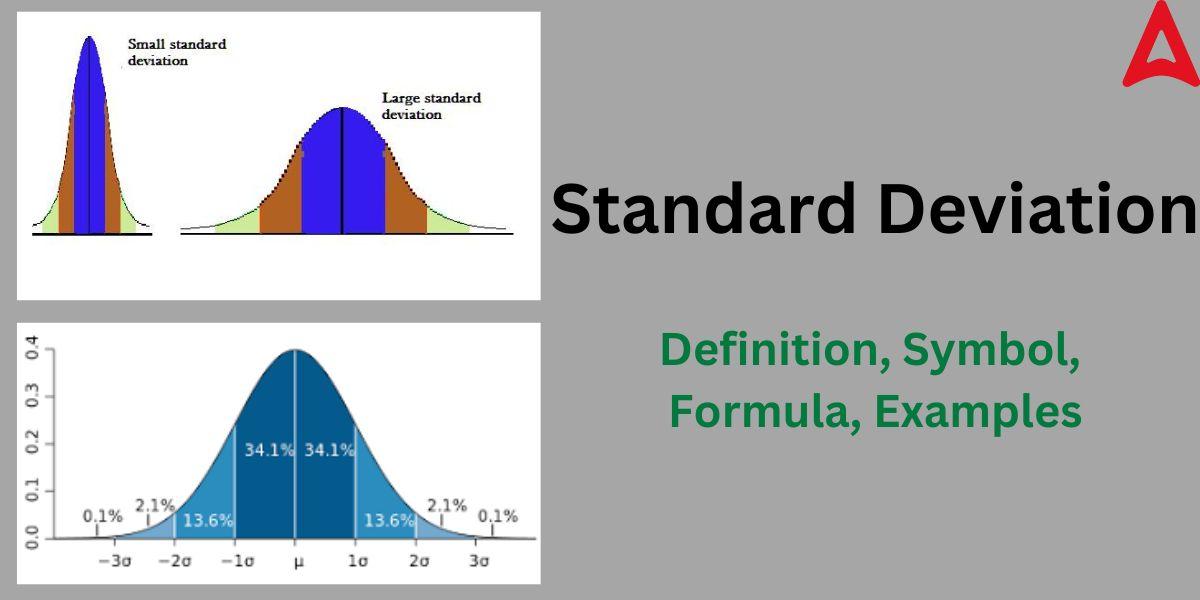
To build on this, let's read about how to calculate and interpret standard deviation in a business context. This article also introduces the concept of variance, which is simply the standard deviation squared. Standard deviation is usually preferred for reporting because it's in the same units as the original data, making it easier to interpret.

3. Practical Application: Sample vs. Population in Excel

In your work, you'll rarely have data for an entire population (e.g., all of your company's customers for all time). Instead, you'll almost always be working with a sample (e.g., customers from the last 30 days, users who saw a specific ad).

This distinction is crucial because the formula for standard deviation is slightly different for a sample versus a population. Thankfully, tools like Excel handle this for you, but you need to tell it which one to use.

• STDEV.P(): Calculates the standard deviation for a Population.
• STDEV.S(): Calculates the standard deviation for a Sample. (You will use this one most of the time).

To see how this works in practice, let's review a guide that walks through an example using Excel.

The ability to take a raw set of numbers in a spreadsheet, calculate the mean and standard deviation, and then articulate what they mean for the business is a fundamental skill for a BA. For example, reporting that "Average daily sales are $975" is useful, but stating that "Average daily sales are $975 with a standard deviation of $440" tells a much richer story about high volatility and potential risks in inventory management.

Conclusion

Congratulations on taking your first step into business analytics! While simple, these concepts are the foundation upon which more complex analyses are built. Mastering them allows you to summarize complex data and begin telling a clear story with numbers.

Key Takeaways:

• Central Tendency describes the "typical" value in a dataset.
  • Mean is the average but is sensitive to outliers.
  • Median is the middle value and is robust to outliers, making it better for skewed data.
• Standard Deviation measures the spread or variability of data around the mean. A low SD means high consistency; a high SD means high volatility.
• For a BA, it's not just about calculation but interpretation. A large gap between mean and median, or a high standard deviation, are signals that require further investigation.
• In practice, you'll mostly work with samples, so you should use the sample standard deviation formula (STDEV.S in Excel).

Preview of the Next Lesson:

Now that you can describe a single set of data, we'll move on to comparing data over time. In the next lesson, you will learn how to calculate and interpret cohort retention rates to analyze user behavior over time. This is a powerful technique used to measure user engagement and the long-term health of a product or service.