The Jacobian Matrix

Hello! In our previous lesson, we established the concept of the gradient for scalar-valued functions ( $f : R^{n} \to R$ ). We saw that the gradient, $\nabla f$ , is a vector of partial derivatives that points in the direction of steepest ascent and allows us to linearly approximate the function's change via the differential $df = (\nabla f)^{T} d x$ .

This lesson extends that crucial idea to vector-valued functions, those of the form $f : R^{n} \to R^{m}$ , which take a vector as input and produce a vector as output. This is the standard scenario in deep learning, where each layer of a network can be seen as a vector-valued function. The derivative of such a function is no longer a vector, but a matrix called the Jacobian matrix.

Our goal in this lesson is to understand what the Jacobian represents and, most importantly, how to compute it for a given vector-valued function.

1. What is the Jacobian? The Intuitive View

Just as the derivative of a single-variable function gives the slope of the tangent line, the Jacobian matrix gives us the best linear transformation that approximates a complex, non-linear vector function near a specific point. It tells us how a small change in the input vector is transformed into a change in the output vector.

The best way to build this intuition is to see it visually. The following video from Khan Academy does an excellent job of explaining this concept. It shows how the columns of the Jacobian matrix correspond to where the basis vectors of the input space land after being transformed.

The Jacobian matrix

Watch this video to develop a strong geometric intuition for the Jacobian. It explains how a nonlinear transformation looks linear when you zoom in on a point, and how the Jacobian matrix captures that local linear behavior.

Watch the entire video (about 6 minutes). Pay close attention to how a tiny step in the x-direction and a tiny step in the y-direction in the input space determine the two columns of the Jacobian matrix in the output space.

As the video illustrates, for a function $f : R^{2} \to R^{2}$ , the Jacobian is a 2x2 matrix that describes the local stretching, rotating, and shearing of the space.

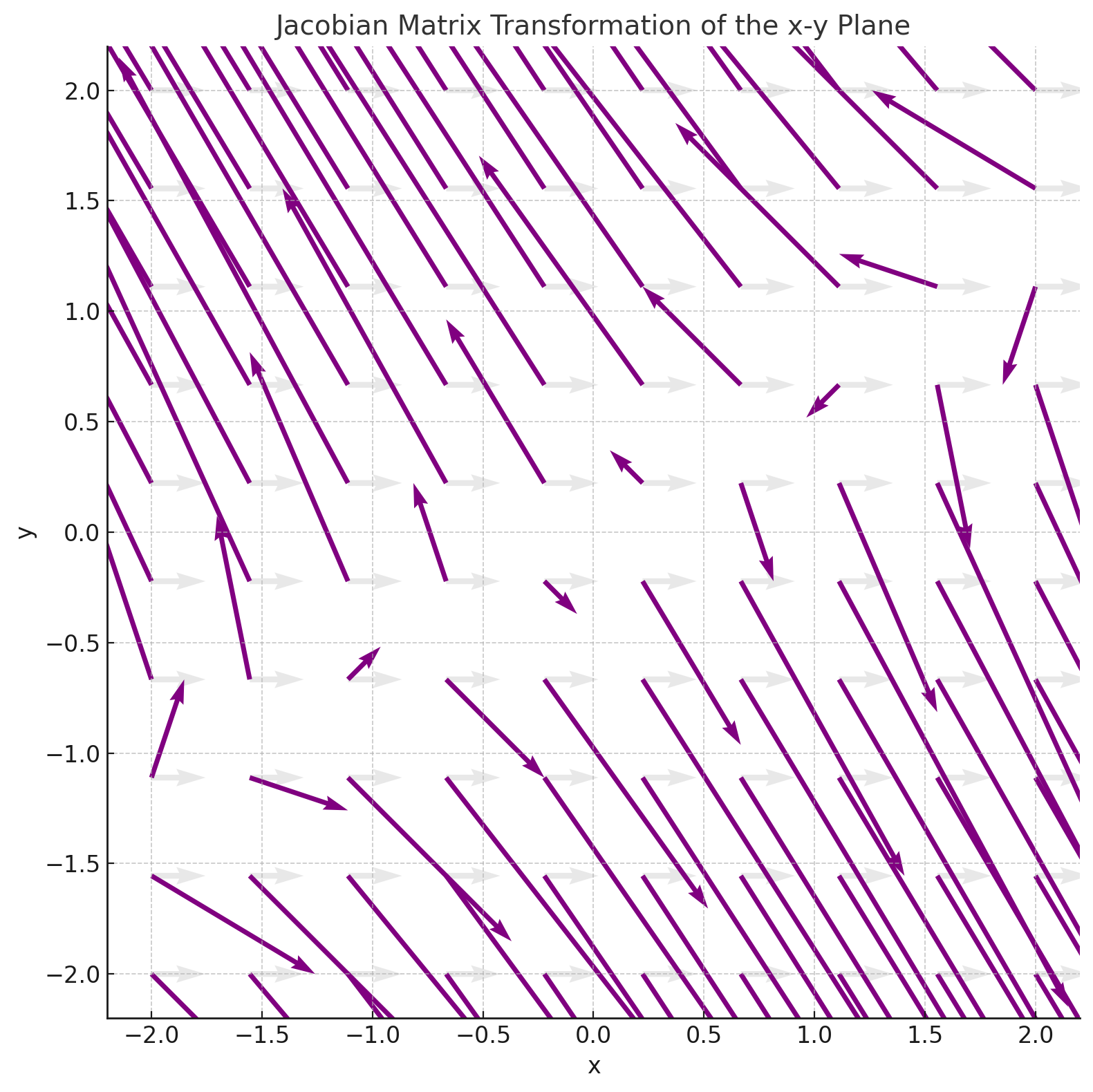
Jacobian Matrix Transformation of the x-y Plane — This image visualizes the effect of a transformation across the x-y plane. The light gray arrows are the original vectors at different points, and the purple arrows are the results of applying the Jacobian matrix at those points. Notice how the transformation's effect (the purple arrows) changes depending on the location, reflecting that the Jacobian itself can be a function of the input variables.

2. The Formal Definition and Computation

Now, let's formalize the structure of the Jacobian matrix. Consider a vector function $f : R^{n} \to R^{m}$ defined as:

f (x) = f_{1} (x_{1}, \dots, x_{n}) f_{2} (x_{1}, \dots, x_{n}) ⋮ f_{m} (x_{1}, \dots, x_{n})

Here, each $f_{i}$ is a scalar-valued function that gives the $i$ -th component of the output vector.

The Jacobian matrix of $f$ with respect to $x$ , denoted $J_{f}$ or $\frac{d f}{d x}$ , is the $m \times n$ matrix of all first-order partial derivatives.

J_{f} = \frac{\partial f _{1}}{\partial x _{1}} \frac{\partial f _{2}}{\partial x _{1}} ⋮ \frac{\partial f _{m}}{\partial x _{1}} \frac{\partial f _{1}}{\partial x _{2}} \frac{\partial f _{2}}{\partial x _{2}} ⋮ \frac{\partial f _{m}}{\partial x _{2}} \dots \dots ⋱ \dots \frac{\partial f _{1}}{\partial x _{n}} \frac{\partial f _{2}}{\partial x _{n}} ⋮ \frac{\partial f _{m}}{\partial x _{n}}

In a more compact form, the entry at row $i$ and column $j$ is $(J_{f})_{ij} = \frac{\partial f _{i}}{\partial x _{j}}$ .

Connecting to the Gradient

Notice the structure of the Jacobian. The first row contains all the partial derivatives of the first component function, $f_{1}$ . The second row contains all the partial derivatives of $f_{2}$ , and so on.

Recall from our previous lesson that we defined the gradient of a scalar function, $\nabla f$ , as a column vector of its partial derivatives. The rows of the Jacobian matrix are therefore the transposes of the gradients of the component functions:

J_{f} = (\nabla f_{1})^{T} (\nabla f_{2})^{T} ⋮ (\nabla f_{m})^{T}

This definition neatly organizes the derivatives of a vector function into a matrix.

This specific layout, an $m \times n$ matrix where rows correspond to output functions, is known as the numerator layout and is common in mathematics and deep learning literature. You might also encounter the denominator layout (the transpose of this matrix), which is more common in physics and some engineering fields. Being aware of both conventions is important. For this course, we will stick to the numerator layout for Jacobians.

3. Step-by-Step Example

Let's compute the Jacobian for a concrete example. This is a purely mechanical process once you understand the definition. You simply need to calculate each partial derivative and place it in the correct spot in the matrix.

The next video from Khan Academy walks through the exact calculation for the function used in the first video.

Computing a Jacobian matrix

This video demonstrates the computational steps to find the Jacobian matrix for a specific function and evaluate it at a point.

Watch the video up to the 2:57 mark. Follow along as each of the four partial derivatives is calculated and placed into the 2x2 Jacobian matrix. Then, see how the numerical Jacobian is found by substituting the coordinates of a specific point.

Let's do one more example ourselves.

Example: Polar to Cartesian Coordinates

Consider the function $f : R^{2} \to R^{2}$ that converts polar coordinates $(r, θ)$ to Cartesian coordinates $(x, y)$ . Our input vector is $(r θ)$ . The function is:

f (r, θ) = (x (r, θ) y (r, θ)) = (r cos θ r sin θ)

Here, $f_{1} (r, θ) = r cos θ$ and $f_{2} (r, θ) = r sin θ$ . The Jacobian is a 2x2 matrix:

J_{f} = (\frac{\partial f _{1}}{\partial r} \frac{\partial f _{2}}{\partial r} \frac{\partial f _{1}}{\partial θ} \frac{\partial f _{2}}{\partial θ})

Now we compute the four partial derivatives:

$\frac{\partial f _{1}}{\partial r} = \frac{\partial}{\partial r} (r cos θ) = cos θ$
$\frac{\partial f _{1}}{\partial θ} = \frac{\partial}{\partial θ} (r cos θ) = - r sin θ$
$\frac{\partial f _{2}}{\partial r} = \frac{\partial}{\partial r} (r sin θ) = sin θ$
$\frac{\partial f _{2}}{\partial θ} = \frac{\partial}{\partial θ} (r sin θ) = r cos θ$

Assembling them gives the Jacobian matrix:

J_{f} (r, θ) = (cos θ sin θ - r sin θ r cos θ)

Test your understanding!

Find the Jacobian matrix for the function $g : R^{3} \to R^{2}$ defined by:

g (x, y, z) = (x^{2} + e^{y} y z - sin (x))

Show answer

The function has two component functions: $g_{1} (x, y, z) = x^{2} + e^{y}$ and $g_{2} (x, y, z) = y z - sin (x)$ . The input vector has 3 components and the output has 2, so the Jacobian will be a $2 \times 3$ matrix.

J_{g} = (\frac{\partial g _{1}}{\partial x} \frac{\partial g _{2}}{\partial x} \frac{\partial g _{1}}{\partial y} \frac{\partial g _{2}}{\partial y} \frac{\partial g _{1}}{\partial z} \frac{\partial g _{2}}{\partial z})

Computing the partials for the first row (from $g_{1}$ ):

$\frac{\partial g _{1}}{\partial x} = 2 x$
$\frac{\partial g _{1}}{\partial y} = e^{y}$
$\frac{\partial g _{1}}{\partial z} = 0$

Computing the partials for the second row (from $g_{2}$ ):

$\frac{\partial g _{2}}{\partial x} = - cos (x)$
$\frac{\partial g _{2}}{\partial y} = z$
$\frac{\partial g _{2}}{\partial z} = y$

The Jacobian matrix is:

J_{g} (x, y, z) = (2 x - cos (x) e^{y} z 0 y)

For a concise, text-based summary of these concepts, the following article is an excellent reference.

The Matrix Calculus You Need For Deep Learning

This article provides a clear, formal definition of the Jacobian by framing it as a collection of gradients. It also explicitly discusses the different layout conventions, which is very helpful.

Read the sections 'Matrix calculus' and 'Generalization of the Jacobian'. Notice how it defines the Jacobian by stacking the gradients of the component functions. This reinforces the connection we made earlier.

Conclusion

In this lesson, we have generalized the concept of a derivative from scalar functions to vector functions, leading us to the Jacobian matrix.

Key Takeaways:

The Jacobian matrix is the best linear approximation of a vector-valued function $f : R^{n} \to R^{m}$ at a point.
It is an $m \times n$ matrix where the entry $(J)_{ij}$ is the partial derivative of the $i$ -th output component with respect to the $j$ -th input component, $\frac{\partial f _{i}}{\partial x _{j}}$ .
The rows of the Jacobian are the transposed gradients of the function's scalar components: $J_{f} = [(\nabla f_{1})^{T}, \dots, (\nabla f_{m})^{T}]^{T}$ .
Computing the Jacobian is a systematic process of calculating all the necessary partial derivatives and arranging them into a matrix.

Preview of the Next Lesson:

Now that we can find the derivative of a single vector-valued function, the next logical step is to consider compositions of functions, like $h (x) = g (f (x))$ . This is exactly what a multi-layer neural network is. To find the derivative of such a composite function, we need a version of the chain rule that works for Jacobians. This will be the topic of our next lesson, and it is the key to the backpropagation algorithm in deep learning.

Recommended resources

1. What is the Jacobian? The Intuitive View

2. The Formal Definition and Computation

Connecting to the Gradient

3. Step-by-Step Example

Conclusion