Chain Rule for Vector and Matrix Derivatives

1. From Scalar to Vector Chain Rule

Let's begin by recalling the single-variable chain rule you know from introductory calculus. If you have a composition of functions, say $y=g(u)$ where $u=f(x)$, the derivative of $y$ with respect to $x$ is given by:

You find the derivative of the "outer" function with respect to its input, multiply it by the derivative of the "inner" function, and substitute to express the result in terms of $x$.

We can generalize this to vector-valued functions. Suppose we have a composition $\mathbf{y}=\mathbf{g}(\mathbf{u})$ and $\mathbf{u}=\mathbf{f}(\mathbf{x})$, where $\mathbf{x}$, $\mathbf{u}$, and $\mathbf{y}$ are vectors. The derivatives of these functions are their Jacobian matrices. The chain rule in this context becomes a product of these matrices.

The vector chain rule is:

This looks identical to the scalar version, but the terms are now Jacobians. Let's check the dimensions to see why this works.

• If $\mathbf{f}:{\mathbb{R}}^n\to {\mathbb{R}}^p$, then its Jacobian $\frac{\partial \mathbf{u}}{\partial \mathbf{x}}$ is a $p\times n$ matrix.
• If $\mathbf{g}:{\mathbb{R}}^p\to {\mathbb{R}}^m$, then its Jacobian $\frac{\partial \mathbf{y}}{\partial \mathbf{u}}$ is an $m\times p$ matrix.

The product $\frac{\partial \mathbf{y}}{\partial \mathbf{u}}\frac{\partial \mathbf{u}}{\partial \mathbf{x}}$ is an $(m\times p)\times (p\times n)$ matrix multiplication, which results in an $m\times n$ matrix. This is exactly the correct size for the Jacobian of the composite function $\mathbf{h}(\mathbf{x})=\mathbf{g}(\mathbf{f}(\mathbf{x}))$, which maps ${\mathbb{R}}^n\to {\mathbb{R}}^m$.

The following article gives a clear explanation of this rule.

2. A Computational View: Backpropagation and Graphs

While the matrix multiplication formula is correct, it can be cumbersome. For the complex, deeply nested functions found in neural networks, a more algorithmic approach is needed. This is where the concept of a computational graph comes in.

A computational graph represents a function as a directed graph where nodes are operations (like addition, matrix multiplication, or an activation function) and edges represent the flow of data.

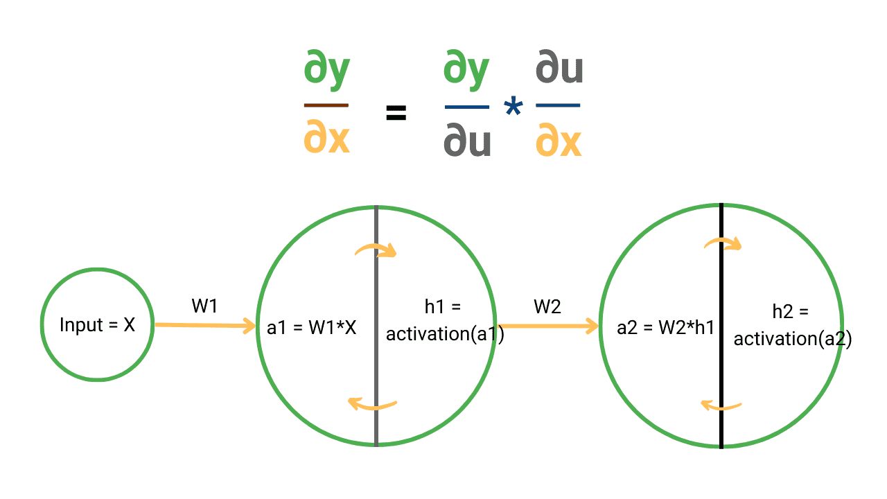
The process of using the chain rule on such a graph is called backpropagation. It consists of two passes:

1. Forward Pass: We feed the input $\mathbf{x}$ into the graph and compute the value at each node until we get the final output. This is just evaluating the function.
2. Backward Pass: We start at the final output and work backward. At each node, we calculate the derivative of the final output with respect to that node's output. The chain rule provides a simple, local recipe for this: multiply the incoming "upstream" gradient by the "local" gradient of the node itself.

The following video brilliantly explains this process.

As the video shows, the chain rule at each node is:
downstream_gradient = upstream_gradient * local_gradient

Now, let's see how this works with vectors, which is the scenario in deep learning.

• The local gradient of a node is its Jacobian matrix.
• The upstream gradient (the derivative of the final scalar loss with respect to the node's vector output) is a vector.
• The multiplication becomes a matrix-vector product.

Let's continue with the same video to see this generalization.

The video makes a critical point for computational efficiency: in practice, we almost never explicitly construct the full, dense Jacobian matrix. For most operations in neural networks, the Jacobian is very sparse (e.g., diagonal for element-wise operations) or has a regular structure. The backpropagation algorithm implements an efficient implicit Jacobian-vector product without ever forming the matrix itself. This insight is key to making deep learning scalable.

3. A Worked Example

Let's apply these ideas to a concrete problem. Consider a simple linear layer followed by a squared norm, which is a common setup for a loss function.

• Let $\mathbf{x}\in {\mathbb{R}}^n$ be an input vector.
• Let $W\in {\mathbb{R}}^{m\times n}$ be a weight matrix.
• The intermediate variable is $\mathbf{y}=W\mathbf{x}$, so $\mathbf{y}\in {\mathbb{R}}^m$.
• The final output is a scalar loss $L=||\mathbf{y}|{|}^2={\mathbf{y}}^T\mathbf{y}$.

Our goal is to find the gradient of the loss with respect to the input, $\frac{\partial L}{\partial \mathbf{x}}$.

We can decompose this into a two-step computational graph: $\mathbf{x}\stackrel{f}{\to }\mathbf{y}\stackrel{g}{\to }L$.
The chain rule states:

Let's compute each part:

1. "Upstream" Gradient ($\frac{\partial L}{\partial \mathbf{y}}$):
   This is the derivative of a scalar $L=y_1^2+y_2^2+\cdots +y_m^2$ with respect to the vector $\mathbf{y}$. We found this gradient in a previous lesson:

   $$\frac{\partial L}{\partial \mathbf{y}}=({\nabla }_{\mathbf{y}}L{)}^T=(2\mathbf{y}{)}^T=2{\mathbf{y}}^T$$

   This is a $1\times m$ row vector.

2. "Local" Gradient ($\frac{\partial \mathbf{y}}{\partial \mathbf{x}}$):
   This is the derivative of the vector function $\mathbf{y}=W\mathbf{x}$ with respect to the vector $\mathbf{x}$. This is a linear transformation, so its derivative is simply the matrix of the transformation itself:

   $$\frac{\partial \mathbf{y}}{\partial \mathbf{x}}=W$$

   This is an $m\times n$ matrix.

Now, we apply the chain rule by multiplying the two results:

The result is a $(1\times m)\times (m\times n)$ product, giving a $1\times n$ row vector, which is the correct shape for the gradient $\frac{\partial L}{\partial \mathbf{x}}$.

Finally, we substitute $\mathbf{y}=W\mathbf{x}$ back in to get the final expression in terms of the input $\mathbf{x}$ and parameters $W$:

If we want this as a column vector (the gradient, ${\nabla }_{\mathbf{x}}L$), we simply take the transpose:

This component-wise approach is a powerful and reliable way to handle complex derivatives.

Conclusion

This lesson connected the Jacobian from our last session to the chain rule, providing the machinery to differentiate complex, nested vector functions.

Key Takeaways:

• The chain rule for vector functions, $\frac{\partial \mathbf{y}}{\partial \mathbf{x}}=\frac{\partial \mathbf{y}}{\partial \mathbf{u}}\frac{\partial \mathbf{u}}{\partial \mathbf{x}}$, is a product of Jacobian matrices.
• In deep learning, this process is algorithmically implemented as backpropagation on a computational graph.
• The core idea of backpropagation is a recursive application of the chain rule: each node in the graph computes its "downstream" gradient by multiplying its "local" gradient (Jacobian) with the "upstream" gradient it receives from the next node.
• Efficient implementations use implicit, structured Jacobian-vector products rather than forming dense matrices.

Preview of the Next Lesson:

So far, we have focused exclusively on first-order derivatives (gradients and Jacobians). These are essential for optimization algorithms like gradient descent, as they tell us the direction of steepest ascent. However, to understand the curvature of a function—whether a critical point is a minimum, maximum, or saddle point—we need to look at second-order derivatives. In the next lesson, we will introduce the Hessian matrix, the generalization of the second derivative to multivariate functions, and see how it helps us classify critical points and analyze the convexity of a function.