Classifying Critical Points with the Hessian Matrix

1. From Second Derivative to Hessian Matrix

In single-variable calculus, the second derivative $f^{\prime \prime }(x)$ tells you about the concavity of a function. A positive second derivative at a critical point means a local minimum, while a negative one means a local maximum.

For a scalar-valued function of multiple variables, $f(\mathbf{x})$ where $\mathbf{x}\in {\mathbb{R}}^n$, the second derivative is no longer a single number. It becomes an $n\times n$ matrix called the Hessian matrix.

The Hessian matrix, denoted $H_f$ or ${\nabla }^{2}f$, is the matrix of all second-order partial derivatives of the function $f$. For a function $f(x_1,x_2,\dots ,x_n)$, its Hessian is:

An important property, thanks to Clairaut's theorem, is that if the second partial derivatives are continuous, the order of differentiation doesn't matter (e.g., $\frac{{\partial }^{2}f}{\partial x_1\partial x_2}=\frac{{\partial }^{2}f}{\partial x_2\partial x_1}$). This means the Hessian matrix is symmetric. This symmetry is a crucial property we will leverage throughout our course.

To get comfortable with computing the Hessian, let's work through a concrete example.

2. The Second Derivative Test for Multivariable Functions

Now that we have the Hessian, how do we use it? The process is a direct parallel to the single-variable case:

1. Find the critical points of the function. These are the points where the gradient is the zero vector, $\nabla f(\mathbf{x})=0$. These are our candidates for local minima, maxima, or saddle points.
2. At each critical point, evaluate the Hessian matrix.
3. Analyze the properties of the Hessian matrix at that point to classify it.

The intuition comes from the second-order Taylor expansion of the function $f$ around a critical point ${\mathbf{x}}_0$:

Since $\nabla f({\mathbf{x}}_0)=0$ at a critical point, this simplifies to:

The expression ${\mathbf{h}}^T{H}_f\mathbf{h}$ is a quadratic form. It describes the curvature of the function around ${\mathbf{x}}_0$. The nature of the critical point depends entirely on whether this quadratic form is always positive, always negative, or changes sign as we move in different directions $\mathbf{h}$.

The following video provides an excellent explanation of this core idea.

To summarize the Second Derivative Test: at a critical point ${\mathbf{x}}_0$:

• If the Hessian $H_f({\mathbf{x}}_0)$ is positive definite (i.e., ${\mathbf{h}}^{T}H\mathbf{h}>0$ for all non-zero $\mathbf{h}$), then $f$ has a local minimum at ${\mathbf{x}}_0$.
• If $H_f({\text{mathbfx}}_0)$ is negative definite (i.e., ${\mathbf{h}}^{T}H\mathbf{h}<0$ for all non-zero $\mathbf{h}$), then $f$ has a local maximum at ${\mathbf{x}}_0$.
• If $H_f({\text{mathbfx}}_0)$ is indefinite (i.e., ${\mathbf{h}}^{T}H\mathbf{h}$ takes both positive and negative values), then $f$ has a saddle point at ${\mathbf{x}}_0$.

3. Eigenvalues: The Key to Definiteness

The definitions of definiteness are conceptually clear, but how do we check them in practice? This is where eigenvalues come to the rescue. Since the Hessian is a symmetric matrix, it has real eigenvalues and an orthonormal basis of eigenvectors. This structure gives us a powerful and intuitive way to understand the quadratic form.

Let's explore this connection.

The key insight from the reading is profound: in the direction of an eigenvector $\mathbf{v}$ with eigenvalue $\lambda$, the function $f$ locally behaves like a simple parabola $\frac{\lambda }{2}{t}^2$. This simplifies the entire problem! The complex curvature of a multivariable function can be understood by looking at the simple parabolic curvatures along its principal axes (the eigenvectors).

This leads to a direct and powerful test for definiteness:

• Positive Definite: All eigenvalues are positive (${\lambda }_i>0$).
• Negative Definite: All eigenvalues are negative (${\lambda }_i<0$).
• Indefinite: At least one positive and at least one negative eigenvalue.
• Semi-definite: Some eigenvalues are zero, and the rest are all of the same sign (e.g., ${\lambda }_i\ge 0$ for positive semi-definite).

4. A Practical Test for the 2D Case

While the eigenvalue test is the most fundamental, computing eigenvalues can be tedious. For the common 2-variable case, $f(x,y)$, there is a well-known shortcut using the determinant and the top-left entry of the Hessian. This is likely the "Second Derivative Test" you encountered in Calculus 3.

Let the Hessian at a critical point be $H=\left(\begin{array}{cc}{f}_{xx}& f_{xy}\\ f_{yx}& f_{yy}\end{array}\right)$ and let $D=\det (H)=f_{xx}{f}_{yy}-(f_{xy}{)}^2$.

1. If $D>0$ and $f_{xx}>0$, then $H$ is positive definite $⟹$ local minimum.
2. If $D>0$ and $f_{xx}<0$, then $H$ is negative definite $⟹$ local maximum.
3. If $D<0$, then $H$ is indefinite $⟹$ saddle point.
4. If $D=0$, the test is inconclusive.

Why does this work? The determinant is the product of the eigenvalues ($D={\lambda }_1{\lambda }_2$).

• If $D>0$, the eigenvalues have the same sign. The sign of $f_{xx}$ (which can be related to the trace, ${\lambda }_1+{\lambda }_2$) then tells you if they are both positive or both negative.
• If $D<0$, the eigenvalues must have opposite signs.

The image below beautifully summarizes this test with a concrete example and a 3D plot.

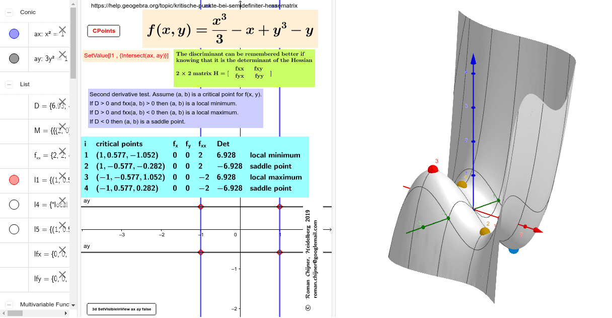
What about the inconclusive case, $D=0$? This implies at least one eigenvalue is zero. In this situation, the quadratic approximation is "flat" in that direction, and we must analyze higher-order terms of the function to classify the point. The functions $f(x,y)=x^4+y^4$ (a minimum) and $g(x,y)=x^3-y^3$ (a saddle) both have a zero Hessian at the origin, showing why the test fails.

Conclusion

In this lesson, we have moved beyond first-order approximations and explored the curvature of multivariable functions using the Hessian matrix.

Key Takeaways:

• The Hessian matrix is the matrix of second partial derivatives of a scalar-valued function. For most functions we care about, it is symmetric.
• The Second Derivative Test allows us to classify critical points (where $\nabla f=0$) as local minima, maxima, or saddle points.
• The classification depends on the definiteness of the Hessian at the critical point, which is fundamentally determined by the signs of its eigenvalues.
  • All positive eigenvalues $⟹$ Local Minimum.
  • All negative eigenvalues $⟹$ Local Maximum.
  • A mix of positive and negative eigenvalues $⟹$ Saddle Point.
• For 2D functions, a practical shortcut using the Hessian's determinant provides a quick way to classify points.

Preview of the Next Lesson:

We've established that a positive definite Hessian signals a local minimum. In our next lesson, we will elevate this concept. We'll see that if a function's Hessian is positive definite everywhere in its domain, not just at a critical point, the function has a special property called convexity. Convex functions, which curve upwards everywhere, are the holy grail of optimization because any local minimum is also a global minimum. This property is absolutely central to many optimization algorithms in machine learning.