Gradients of Scalar Functions

1. From Scalar Derivatives to Gradients

Before we jump into vectors and matrices, let's briefly revisit the core idea of a derivative in single-variable calculus. The derivative $f^{\prime }(x)$ gives us the best linear approximation of a function $f$ near a point $x_0$. This idea of linearization is the foundation we will build upon.

To see a great review of this concept and how it sets the stage for everything that follows, please watch the beginning of the following lecture by MIT's Alan Edelman.

As the video explains, the relationship $dy=f^{\prime }(x)dx$ is central. It tells us how a small perturbation $dx$ in the input is linearly transformed into a perturbation $dy$ in the output. We are now going to extend this to functions whose inputs are not single numbers, but vectors.

2. The Gradient: Differentiating with Respect to a Vector

Let's consider a function $f$ that maps a vector $\mathbf{x}\in {\mathbb{R}}^n$ to a single scalar, written $f:{\mathbb{R}}^n\to \mathbb{R}$. A common example in machine learning is a "cost" or "loss" function, which measures how poorly a model is performing. The input vector $\mathbf{x}$ could represent all the tunable weights in the model.

The gradient of $f$ with respect to $\mathbf{x}$ is the vector containing all the partial derivatives of $f$. We denote it as ${\nabla }_{\mathbf{x}}f(\mathbf{x})$.

Notice that the gradient is a column vector with the same dimension as the input vector $\mathbf{x}$. This is a common convention in machine learning known as denominator layout.

Geometric Intuition

What does this vector represent? The gradient $\nabla f$ evaluated at a point ${\mathbf{x}}_0$ points in the direction of the steepest ascent of the function at that point. Conversely, the negative gradient, $-\nabla f$, points in the direction of steepest descent. This is precisely why gradients are crucial for optimization: to minimize a function, we just need to follow the direction of its negative gradient.

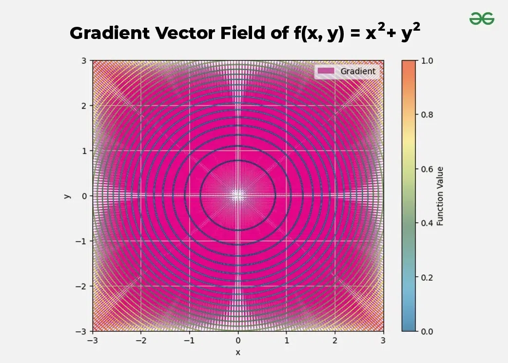
Computation Method 1: Element-wise Derivation

The most direct way to compute a gradient is to calculate each partial derivative $\frac{\partial f}{\partial x_i}$ one by one, treating all other components of $\mathbf{x}$ as constants.

Example: The Squared L2 Norm

Let $f(\mathbf{x})=\Vert \mathbf{x}{\Vert }_2^2={\mathbf{x}}^T\mathbf{x}=x_1^2+x_2^2+\cdots +x_n^2$.
To find the gradient, we compute the partial derivative with respect to an arbitrary component $x_k$:

The derivative is zero for all terms where $i\ne k$. The only non-zero term is when $i=k$, which gives $\frac{\partial }{\partial x_k}(x_k^2)=2x_k$.
Assembling these into a vector, we get:

This element-wise approach is straightforward, but it can become very tedious.

Computation Method 2: The Differential Approach

A more powerful and elegant method, especially for complex functions, is to use differentials, just as Alan Edelman did in the video. We generalize the scalar linearization $df=f^{\prime }(x)dx$ to vectors. The total differential of $f(\mathbf{x})$ is the dot product of the gradient with the differential vector $d\mathbf{x}$:

Our strategy will be to compute $df$ using calculus rules for vectors and matrices, and then manipulate the expression into the form (something)^T d**x**. That "something" will be our gradient.

Let's re-do our example $f(\mathbf{x})={\mathbf{x}}^T\mathbf{x}$ using this approach. We'll use the product rule, which for vectors states $d({\mathbf{u}}^T\mathbf{v})=(d{\mathbf{u}}^T)\mathbf{v}+{\mathbf{u}}^T(d\mathbf{v})$.

1. Find the differential: $$df=d({\mathbf{x}}^T\mathbf{x})=(d{\mathbf{x}}^T)\mathbf{x}+{\mathbf{x}}^T(d\mathbf{x})$$
2. Simplify: Note that $(d{\mathbf{x}}^T)\mathbf{x}$ is a scalar (a $1\times 1$ matrix). The transpose of a scalar is itself. So, $(d{\mathbf{x}}^T)\mathbf{x}=((d{\mathbf{x}}^T)\mathbf{x}{)}^T={\mathbf{x}}^T(d\mathbf{x})$. The two terms are identical. $$df={\mathbf{x}}^T(d\mathbf{x})+{\mathbf{x}}^T(d\mathbf{x})=2{\mathbf{x}}^{T}d\mathbf{x}$$
3. Identify the gradient: We have our expression in the form $df=(\text{something}{)}^{T}d\mathbf{x}$. $$df=\underset{\text{matches }(\nabla f{)}^T}{\underbrace{(2\mathbf{x}{)}^T}}d\mathbf{x}$$ By comparing the forms, we can directly identify the gradient: ${\nabla }_{\mathbf{x}}f(\mathbf{x})=2\mathbf{x}$.

This method avoids breaking the vector down into its components. The next segment of the Edelman video masterfully demonstrates this technique.

3. Differentiating with Respect to a Matrix

Now we extend the concept to functions that take a matrix $X\in {\mathbb{R}}^{m\times n}$ and return a scalar, $f:{\mathbb{R}}^{m\times n}\to \mathbb{R}$. The gradient is now a matrix of the same size as $X$, where each element is a partial derivative.

To use our differential method, we need a way to turn a matrix expression back into a scalar. The dot product worked for vectors. For matrices, the analogous operation is the trace.

The Trace Operator

The trace of a square matrix, denoted $\mathrm{tr}(A)$, is the sum of its diagonal elements. For our purposes, it has two crucial properties:

1. Linearity: $\mathrm{tr}(A+B)=\mathrm{tr}(A)+\mathrm{tr}(B)$ and $\mathrm{tr}(cA)=c\cdot \mathrm{tr}(A)$.
2. Cyclic Property: $\mathrm{tr}(ABC)=\mathrm{tr}(BCA)=\mathrm{tr}(CAB)$. You can cycle the matrices in a product without changing the trace, as long as the dimensions remain compatible.

The identity that connects the differential $df$ to the gradient ${\nabla }_{X}f$ is:

Our strategy remains the same: calculate $df$ using calculus rules, then massage the expression into the form $\mathrm{tr}((\text{something}{)}^{T}dX)$. That "something" will be the gradient.

Let's see this in action with the help of the final part of the video.

As shown in the video, for $f(A)=\mathrm{tr}(A^2)$, we found that $df=\mathrm{tr}(2A^{T}dA)$. By matching this to the identity $df=\mathrm{tr}(({\nabla }_{A}f{)}^{T}dA)$, we can conclude that ${\nabla }_{A}f=(2A^T{)}^T=2A$. Correction: The video shows ${\nabla }_{A}f=2A^T$, let's re-verify the derivation.

Let's retrace the steps from the video for $f(A)=\mathrm{tr}(A^2)$:

1. $df=d(\mathrm{tr}(A^2))=\mathrm{tr}(d(A^2))$
2. $df=\mathrm{tr}(dA\cdot A+A\cdot dA)$
3. $df=\mathrm{tr}(dA\cdot A)+\mathrm{tr}(A\cdot dA)$
4. Using the cyclic property on the first term: $\mathrm{tr}(dA\cdot A)=\mathrm{tr}(A\cdot dA)$.
5. So, $df=2\mathrm{tr}(A\cdot dA)$.
6. To match the form $\mathrm{tr}((\nabla f{)}^{T}dA)$, we identify $(\nabla f{)}^T$ with $2A$.
7. Therefore, $\nabla f=(2A{)}^T=2A^T$.

The video's result is correct. This elegant, element-free approach is extremely useful. For a more direct, text-based explanation of these definitions, you can refer to the following resources.

Conclusion

In this lesson, we have taken our first and most important step into matrix calculus. We have defined the gradient for functions of vectors and matrices, which is the cornerstone of optimization in machine learning.

Key Takeaways:

• The gradient ($\nabla f$) of a scalar-valued function $f$ is the vector or matrix of its partial derivatives.
• The gradient has the same shape as the input variable (using denominator layout convention).
• Geometrically, the gradient points in the direction of the function's steepest ascent.
• Gradients can be computed element-by-element, but a more powerful differential method treats vectors and matrices as whole objects.
• The key relations for the differential method are:
  • For vectors: $df=({\nabla }_{\mathbf{x}}f{)}^{T}d\mathbf{x}$
  • For matrices: $df=\mathrm{tr}(({\nabla }_{X}f{)}^{T}dX)$
• The product rule and the cyclic property of the trace are essential tools for this approach.

Preview of the Next Lesson:

We've dealt with functions that output a single scalar. But what if a function outputs a whole vector? For example, each layer in a neural network transforms an input vector into an output vector. To handle derivatives of such functions, we need to generalize the gradient to the Jacobian matrix. That will be our next topic.