SVD for Rank, Kernel, and Image

1. The Four Fundamental Subspaces

Before we dive into the SVD's role, let's briefly revisit the four fundamental subspaces associated with any $m\times n$ matrix $A$. You've encountered some of these concepts before, like span and solution sets, but let's organize them.

• Column Space (or Image), $\mathcal{C}(A)$: The set of all possible output vectors. It's the span of the columns of $A$. A vector $\mathbf{b}$ is in the column space if the equation $A\mathbf{x}=\mathbf{b}$ has a solution. It is a subspace of ${\mathbb{R}}^m$.
• Null Space (or Kernel), $\mathcal{N}(A)$: The set of all input vectors that are mapped to the zero vector. It's the set of all solutions to the equation $A\mathbf{x}=0$. It is a subspace of ${\mathbb{R}}^n$.
• Row Space, $\mathcal{C}(A^T)$: The span of the rows of $A$. It is a subspace of ${\mathbb{R}}^n$.
• Left Null Space, $\mathcal{N}(A^T)$: The null space of the transpose of $A$. It is a subspace of ${\mathbb{R}}^m$.

These four spaces are not independent; they are linked by deep and elegant relationships. The following diagram, famously drawn by Gilbert Strang, provides a powerful mental map of how they relate.

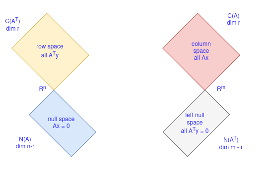
The dimension of both the column space and the row space is the rank of the matrix, denoted by $r$. The diagram also shows the dimensions of the null spaces, which are given by what we'll later know as the Rank-Nullity Theorem.

The amazing thing about SVD is that it gives us an orthonormal basis for all four of these subspaces.

2. Reading the Subspaces from SVD

Let's see how the SVD factorization $A=U\Sigma V^T$ cleanly separates these subspaces.

The most direct and perhaps most important property that SVD reveals is the rank of the matrix.

The rank of a matrix $A$ is equal to the number of its non-zero singular values.

This is because the singular values represent the "stretching" factors of the transformation. If a singular value is zero, it means the transformation collapses that dimension entirely. The number of dimensions that survive the transformation is the rank.

To understand how SVD reveals the bases for the subspaces, it's helpful to expand the SVD equation. Let's assume $A$ is an $m\times n$ matrix of rank $r$. This means there are $r$ non-zero singular values. We can write the equation $A=U\Sigma V^T$ as $AV=U\Sigma$. Let's look at what this means for each column vector ${\mathbf{v}}_i$ of $V$:

By looking at this column by column, we get two distinct cases:

1. For $i=1,\dots ,r$: $A{\mathbf{v}}_i={\sigma }_i{\mathbf{u}}_i$
2. For $i=r+1,\dots ,n$: $A{\mathbf{v}}_i=0$ (since the corresponding singular values are zero)

These two simple equations are incredibly powerful. They tell us exactly where SVD places the basis vectors for the fundamental subspaces.

The following reading explains this derivation clearly and summarizes the results.

Summary of SVD and the Four Subspaces

Let's consolidate the key findings from the reading. For an $m\times n$ matrix $A$ of rank $r$, with SVD $A=U\Sigma V^T$:

• Column Space $\mathcal{C}(A)$: The first $r$ columns of $U$, $\{{\mathbf{u}}_1,\dots ,{\mathbf{u}}_r\}$, form an orthonormal basis for the column space.
  • Intuition: The equation $A{\mathbf{v}}_i={\sigma }_i{\mathbf{u}}_i$ shows that the outputs of the transformation are spanned by these ${\mathbf{u}}_i$ vectors.
• Null Space $\mathcal{N}(A)$: The last $n-r$ columns of $V$, $\{{\mathbf{v}}_{r+1},\dots ,{\mathbf{v}}_n\}$, form an orthonormal basis for the null space.
  • Intuition: The equation $A{\mathbf{v}}_i=0$ for these vectors is the very definition of the null space.
• Row Space $\mathcal{C}(A^T)$: The first $r$ columns of $V$, $\{{\mathbf{v}}_1,\dots ,{\mathbf{v}}_r\}$, form an orthonormal basis for the row space.
• Left Null Space $\mathcal{N}(A^T)$: The last $m-r$ columns of $U$, $\{{\mathbf{u}}_{r+1},\dots ,{\mathbf{u}}_m\}$, form an orthonormal basis for the left null space.

This is a remarkable result. The SVD calculation, which we perform for geometric reasons, simultaneously gives us a complete, orthonormal description of the matrix's fundamental structure.

3. A Concrete Example

Let's solidify this with a practical example. As a computer science student, you'll appreciate that libraries like NumPy can compute the SVD in a single line of code, after which we can just "read off" the subspaces.

Consider the following Python code, which analyzes a 5x5 matrix A.

import numpy as np
np.set_printoptions(precision=2, suppress=True)

# Define a 5x5 matrix of rank 2
A = np.array([[1, 2, 3, 4, 5],
              [2, 4, 6, 8, 10],
              [3, 5, 8, 11, 14],
              [4, 7, 11, 15, 19],
              [5, 9, 14, 19, 24]])

# Compute the SVD
U, S, Vt = np.linalg.svd(A)

# Compute the rank
rank = np.linalg.matrix_rank(A)

print("Rank of matrix A:", rank)
print("\nSingular values (S):", S)

# Identify the basis vectors
# Note: In Python, we use slicing. V is already transposed in the output, so we take rows.
basis_col_space = U[:, :rank]
basis_left_null_space = U[:, rank:]

basis_row_space = Vt[:rank, :].T  # Transpose to get column vectors
basis_null_space = Vt[rank:, :].T # Transpose to get column vectors

print("\nShape of basis for Column Space:", basis_col_space.shape)
print("Shape of basis for Null Space:", basis_null_space.shape)

Running this code would produce output like this:

Rank of matrix A: 2

Singular values (S): [50.84 2.39 0.   0.   0.  ]

Shape of basis for Column Space: (5, 2)
Shape of basis for Null Space: (5, 3)

Let's interpret this result:

• The rank is 2, which matches the number of non-zero singular values (50.84 and 2.39).
• The column space is a 2-dimensional subspace of ${\mathbb{R}}^5$. An orthonormal basis for it is given by the first 2 columns of the U matrix.
• The null space is a 3-dimensional subspace of ${\mathbb{R}}^5$ (since $n=5$ and $r=2$, the dimension is $n-r=3$). An orthonormal basis is given by the last 3 columns of the V matrix (or last 3 rows of Vt).

Conclusion

In this lesson, we transitioned from the geometric view of SVD to its structural interpretation. You now have a powerful and practical method to dissect any matrix and understand its fundamental properties.

Key Takeaways:

• The SVD, $A=U\Sigma V^T$, provides orthonormal bases for the four fundamental subspaces of $A$.
• The rank of $A$ is simply the number of non-zero singular values.
• The first $r$ columns of $U$ form an orthonormal basis for the column space (image).
• The last $n-r$ columns of $V$ form an orthonormal basis for the null space (kernel).
• Similarly, the first $r$ columns of $V$ form a basis for the row space, and the last $m-r$ columns of $U$ form a basis for the left null space.

Preview of the Next Lesson:

What happens when a matrix is not invertible? This occurs when its null space is non-trivial (i.e., it has at least one zero singular value), making it impossible to uniquely reverse the transformation. However, for many practical problems in machine learning, like finding the best fit line in linear regression, we still need a way to "solve" systems involving such matrices.

In our next lesson, we will learn how to use the SVD to compute the pseudoinverse of a matrix. This is a generalization of the inverse that provides the best possible solution even for non-invertible or non-square matrices.