SVD: Decoding Matrix Transformations

1. From Complex Transformations to Simple Steps

Any linear transformation can stretch, shrink, shear, or rotate vectors. This can seem complicated. For instance, a shear transformation deforms a square into a parallelogram, which isn't a simple rotation or scaling.

The central idea of SVD's geometric interpretation is that even a complex transformation like a shear becomes a simple stretch/compression if we're allowed to rotate our object first. The SVD gives us the exact rotations needed to make this simplification work for any matrix.

Let's build this intuition with an excellent, jargon-free article.

The key takeaway is powerful: Any linear transformation maps a set of orthonormal input vectors (the columns of $V$) to a set of orthonormal output vectors (the columns of $U$), scaling them by the singular values (the entries of $\Sigma$). Geometrically, this means it transforms a sphere (or circle) into an ellipsoid (or ellipse).

2. Visualizing the Three-Step Process

Let's analyze the transformation of a vector $\mathbf{x}$ by a matrix $A$. The SVD expresses this as $A\mathbf{x}=U\Sigma V^T\mathbf{x}$. Since matrix multiplication is applied from right to left, the process is:

1. First, apply $V^T$: This is the first rotation.
2. Then, apply $\Sigma$: This is the scaling.
3. Finally, apply $U$: This is the second rotation.

The following video by Professor Gilbert Strang provides one of the clearest visual explanations of this process.

This sequence is the heart of the geometric interpretation. Let's capture it with a diagram and formalize the steps.

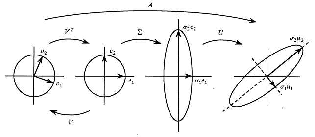
The Breakdown:

1. Rotation 1 ($V^T$): $V$ is an orthogonal matrix whose columns, ${\mathbf{v}}_i$, form an orthonormal basis for the input space. These are the "principal input directions." Applying $V^T$ to a vector $\mathbf{x}$ reorients the space so that these principal directions align with the standard coordinate axes (${\mathbf{e}}_1,{\mathbf{e}}_2,\dots$). The shape (a circle) doesn't change, only its orientation.

2. Scaling ($\Sigma$): $\Sigma$ is a diagonal matrix. It scales the space along each coordinate axis. The component along the first axis is multiplied by ${\sigma }_1$, the second by ${\sigma }_2$, and so on. This is where the circle is stretched or squashed into an ellipse, with its axes lying perfectly along the coordinate axes. The lengths of these semi-axes are the singular values ${\sigma }_i$.

3. Rotation 2 ($U$): $U$ is another orthogonal matrix. Its columns, ${\mathbf{u}}_i$, form an orthonormal basis for the output space, representing the "principal output directions." Applying $U$ takes the axis-aligned ellipse and rotates it to its final orientation in the output space. The axes of the final ellipse now point along the directions of the ${\mathbf{u}}_i$ vectors.

To solidify this, let's look at one more visual walkthrough, which you might appreciate as it uses plots generated from Python code.

3. The Roles of U, Σ, and V

Now we can assign a clear geometric role to each component of the SVD:

• $V$: The columns of $V$ are the principal input directions of $A$. They are an orthonormal basis for the input space with a special property: their images under $A$ ($A{\mathbf{v}}_i$) are orthogonal. They represent the axes of the initial circle that will become the axes of the final ellipse.

• $\Sigma$: The diagonal entries of $\Sigma$ (${\sigma }_i\ge 0$) are the scaling factors or principal stretches. ${\sigma }_i$ is the length of the vector $A{\mathbf{v}}_i$. The largest singular value, ${\sigma }_1$, represents the maximum amount of stretching the transformation $A$ applies to any vector.

• $U$: The columns of $U$ are the principal output directions of $A$. They are an orthonormal basis for the output space that gives the directions of the axes of the final ellipse. Specifically, ${\mathbf{u}}_i$ is the unit vector in the direction of $A{\mathbf{v}}_i$.

The following short video beautifully visualizes the search for these special input vectors that remain orthogonal after the transformation.

Conclusion

In this lesson, we've unveiled the profound geometric meaning behind the Singular Value Decomposition. Instead of just a formula, we can now see $A=U\Sigma V^T$ as a "story" of transformation.

Key Takeaways:

• Any linear transformation represented by a matrix $A$ can be geometrically decomposed into a sequence of rotation ($V^T$), scaling ($\Sigma$), and another rotation ($U$).
• This process transforms an input sphere/circle into an output ellipsoid/ellipse.
• The columns of $V$ are the principal directions of the input space that remain orthogonal after transformation.
• The diagonal entries of $\Sigma$ are the scaling factors along these principal directions.
• The columns of $U$ define the final orientation (the principal axes) of the transformed shape in the output space.

Preview of the Next Lesson:

Now that we understand SVD's construction and its geometric meaning, we are ready to put it to work. In the next lesson, we will see how this powerful decomposition allows us to easily read off fundamental properties of a matrix, such as its rank, kernel (null space), and image (column space), directly from its SVD components.