Pseudoinverse Computation with SVD

1. When the Inverse Fails: The Need for an Alternative

Before we define the pseudoinverse, let's build our intuition about why we need it. Most systems of equations you'll encounter in machine learning are not simple, square, invertible systems. They usually fall into one of two categories.

The following video provides an excellent overview of these cases and motivates the need for a generalized inverse.

To summarize the key ideas from the video:

• Overdetermined Systems (Tall, skinny matrix, $m>n$): We have more equations (data points) than unknowns (features). Think of trying to fit a single straight line perfectly through 100 scattered points. In general, there is no exact solution because the vector $\mathbf{b}$ is unlikely to lie in the column space of $A$.
• Underdetermined Systems (Short, fat matrix, $m<n$): We have fewer equations than unknowns. Think of having two variables but only one equation, like $x+y=5$. There are infinitely many solutions.

In both scenarios, the standard inverse $A^{-1}$ is undefined. We need a new tool that can give us a meaningful, "best" answer in both cases. This tool is the Moore-Penrose pseudoinverse.

2. Constructing the Pseudoinverse from SVD

The beauty of the SVD is that it provides a direct way to construct the pseudoinverse. The logic is wonderfully straightforward.

If we have $A=U\Sigma V^T$ and want to "invert" it to solve for $\mathbf{x}$ in $A\mathbf{x}=\mathbf{b}$, our first instinct might be to invert each component:

Since $U$ and $V$ are unitary matrices, their inverses are simply their transposes ($U^{-1}=U^T$ and $(V^T{)}^{-1}=V$). So, the expression becomes:

This looks promising! The only problem is ${\Sigma }^{-1}$. The matrix $\Sigma$ is generally rectangular and contains zeros on its diagonal, making it non-invertible in the standard sense.

The solution is to define a pseudoinverse of $\Sigma$, denoted ${\Sigma }^{†}$. Here is how you construct it:

1. Start with the $m\times n$ matrix $\Sigma$.
2. Create a new $n\times m$ matrix, ${\Sigma }^{†}$, filled with zeros.
3. For every non-zero singular value ${\sigma }_i$ at position $(i,i)$ in $\Sigma$, place its reciprocal $1/{\sigma }_i$ at position $(i,i)$ in ${\Sigma }^{†}$.

For example, if we have a $3\times 2$ matrix $A$ of rank 2, its $\Sigma$ matrix and its pseudoinverse ${\Sigma }^{†}$ would be:

Notice that ${\Sigma }^{†}$ has the shape of ${\Sigma }^T$.

With this final piece, we can formally define the pseudoinverse of $A$.

Definition: The Pseudoinverse

For a matrix $A$ with SVD $A=U\Sigma V^T$, its pseudoinverse $A^{†}$ is defined as:

The "best" solution to the system $A\mathbf{x}=\mathbf{b}$ is then given by:

We use $\hat{\mathbf{x}}$ (read "x-hat") to signify that this is an estimated or approximate solution, not necessarily an exact one.

The following video walks through this derivation and shows how to calculate the components in practice.

For a supplementary text-based derivation, the following article is also very helpful.

3. The Optimal Nature of the Pseudoinverse Solution

We've repeatedly called $\hat{\mathbf{x}}=A^{†}\mathbf{b}$ the "best" solution. But what does "best" actually mean? The answer depends on which of the two problem cases we are in. The properties of the pseudoinverse solution are precisely what make it so useful in machine learning and optimization.

Let's return to the video by Steve Brunton to see what makes this solution optimal.

Here is a summary of these two crucial properties:

1. For overdetermined systems (more equations than unknowns, usually no solution), the pseudoinverse provides the least squares solution. This means that $\hat{\mathbf{x}}=A^{†}\mathbf{b}$ is the vector $\mathbf{x}$ that minimizes the error between the desired output $\mathbf{b}$ and the actual output $A\mathbf{x}$. Specifically, it minimizes the Euclidean norm of the error vector: $\Vert \mathbf{Ax}-\mathbf{b}{\Vert }_2$. This is the foundation of linear regression.

   Geometrically, $A\hat{\mathbf{x}}$ is the orthogonal projection of the vector $\mathbf{b}$ onto the column space of $A$. It's the closest possible vector to $\mathbf{b}$ that can actually be produced by the transformation $A$.

   
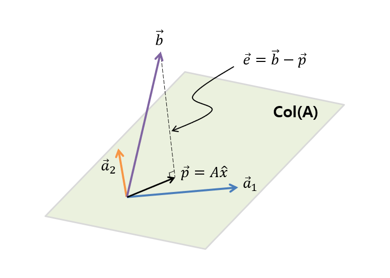
   This image from the angeloyeo.github.io article illustrates the concept. When $\mathbf{b}$ is outside the column space of A (Col(A)), no exact solution exists. The pseudoinverse finds the solution $\hat{x}$ that produces the projection of $\mathbf{b}$ onto Col(A), which is the closest vector in the column space to $\mathbf{b}$.

2. For underdetermined systems (fewer equations than unknowns, infinite solutions), the pseudoinverse provides the minimum norm solution. Of the infinitely many vectors $\mathbf{x}$ that exactly solve $A\mathbf{x}=\mathbf{b}$, the vector $\hat{\mathbf{x}}=A^{†}\mathbf{b}$ is the one with the smallest length (smallest Euclidean norm, $\Vert \mathbf{x}{\Vert }_2$). In many physical or computational systems, this corresponds to the most "efficient" or "simplest" solution.

Conclusion

Today, we've added a powerful and practical tool to our linear algebra toolkit. By leveraging the SVD, we can now find a meaningful solution to any system of linear equations $A\mathbf{x}=\mathbf{b}$, regardless of the shape or rank of $A$.

Key Takeaways:

• The pseudoinverse ($A^{†}$) generalizes the matrix inverse to all matrices, including non-square and singular ones.
• It is computed directly from the SVD components via the formula $A^{†}=V{\Sigma }^{†}{U}^T$.
• The matrix ${\Sigma }^{†}$ is constructed by taking the transpose of $\Sigma$ and replacing the non-zero singular values ${\sigma }_i$ with their reciprocals $1/{\sigma }_i$.
• The solution $\hat{\mathbf{x}}=A^{†}\mathbf{b}$ is "optimal" in two distinct ways:
  • It's the least squares solution for overdetermined systems (minimizing error).
  • It's the minimum norm solution for underdetermined systems (shortest solution vector).

Preview of the Next Lesson:

The concept of a "least squares solution" is not just a mathematical curiosity; it's the engine behind one of the most fundamental algorithms in data science: linear regression. In our next lesson, we will formally define the least squares problem and see how the pseudoinverse provides an elegant and direct method for finding the "best-fit" line through a set of data points.