Low-Rank Matrix Approximation with SVD

Hello! Welcome to the final lesson in our module on Singular Value Decomposition.

In the previous lessons, we've explored the power of SVD to deconstruct any matrix $A$ into its fundamental components: $A = U Σ V^{T}$ . We used this decomposition to understand a matrix's rank, kernel, and image, and even to compute the pseudoinverse, $A^{†} = V Σ^{†} U^{T}$ , which provides the "best" solution to any linear system.

Today, we'll explore another powerful application of SVD that is central to modern data science and machine learning. Our goal is to apply SVD to find the best low-rank approximation of a matrix. This technique is the foundation for everything from data compression and noise reduction to building recommender systems.

1. The "Why": Data Compression and Latent Features

Imagine you have a massive matrix, perhaps representing every pixel in a high-resolution image or the ratings of millions of users for thousands of movies. Storing and performing calculations with such a large matrix can be computationally expensive. What if we could capture the essence of the matrix in a much smaller, simpler form?

This is the core idea behind low-rank approximation. We want to find a new matrix, with a lower rank, that is as close as possible to the original. A lower-rank matrix has fewer linearly independent columns/rows, implying it contains less complex information and can be stored more efficiently.

Understanding SVD's Intuition

This article, 'Understanding SVD's Intuition', gives a great high-level overview of why low-rank approximation is so valuable. It frames SVD as a tool to find 'latent features' hidden in the data.

Please read the sections 'Why Was SVD Developed?', 'What does it mean to find the best approximation of a matrix by a lower-rank matrix?', and 'Application in Dimensionality Reduction'. This will provide the motivation for why we are doing this.

As the article highlights, low-rank approximation helps us:

Compress data: By storing fewer numbers while preserving the main structure.
Filter noise: By discarding the less important, often noisy, components of the data.
Discover latent features: By revealing the underlying patterns that govern the data.

2. SVD as a Sum of Weighted, Rank-One Matrices

To understand how SVD gives us the best approximation, we first need to look at the decomposition in a slightly different way. Instead of a product of three matrices, we can express $A$ as a weighted sum of simpler matrices.

The SVD $A = U Σ V^{T}$ can be rewritten as:

A = i = 1 \sum r σ_{i} u_{i} v_{i}^{T}

where $r$ is the rank of $A$ , $σ_{i}$ is the $i$ -th singular value, $u_{i}$ is the $i$ -th column of $U$ (a left singular vector), and $v_{i}^{T}$ is the $i$ -th row of $V^{T}$ (the transpose of a right singular vector).

Each term in this sum, $u_{i} v_{i}^{T}$ , is an outer product of two vectors, which results in a rank-one matrix. So, the SVD tells us that any matrix can be built by adding together a series of rank-one matrices, each weighted by its corresponding singular value.

Since the singular values are always sorted in descending order ( $σ_{1} \geq σ_{2} \geq \dots \geq σ_{r} > 0$ ), the first term $σ_{1} u_{1} v_{1}^{T}$ is the most significant "piece" of the matrix. The second term adds the next most significant piece, and so on.

Singular Value Decomposition (SVD): Matrix Approximation

Steve Brunton provides an excellent visualization of this concept, showing how the matrix A is constructed piece by piece from its most important components.

Watch the video from 1:30 to 8:17. Focus on how the product U \Sigma V^T is expanded into a sum of outer products and why each of these terms is a rank-one matrix.

3. Truncating the SVD for the Best Approximation

The insight that SVD is a weighted sum of rank-one matrices gives us a straightforward way to create a low-rank approximation. If we want a rank- $k$ approximation (where $k < r$ ), we can simply keep the first $k$ "most important" terms from the sum and discard the rest.

This is called the truncated SVD. The rank- $k$ approximation of $A$ , which we'll call $A_{k}$ , is defined as:

A_{k} = i = 1 \sum k σ_{i} u_{i} v_{i}^{T}

This is equivalent to reconstructing the matrix using only the first $k$ singular values and their corresponding singular vectors:

A_{k} = U_{k} Σ_{k} V_{k}^{T}

Where:

$U_{k}$ is the matrix containing the first $k$ columns of $U$ .
$Σ_{k}$ is the top-left $k \times k$ diagonal matrix of $Σ$ .
$V_{k}^{T}$ is the matrix containing the first $k$ rows of $V^{T}$ .

Low-rank Approximation via SVD — This image illustrates the process of creating a rank-k approximation. We start with the full SVD and effectively set the smaller singular values ($\sigma_{k+1}, \dots, \sigma_r$) to zero, which is the same as truncating the matrices $U$, $\Sigma$, and $V$.

4. The Eckart-Young Theorem: A Guarantee of Optimality

Here's the most important part: the matrix $A_{k}$ we just constructed is not just an approximation; it is the best possible rank-k approximation of $A$ .

This is formally stated by the Eckart-Young-Mirsky Theorem. It guarantees that among all possible matrices of rank $k$ , $A_{k}$ is the one that minimizes the approximation error. The error is typically measured using the Frobenius norm, $∥ A - A_{k} ∥_{F}$ , which is like the Euclidean distance for matrices (the square root of the sum of the squares of all its elements).

Eckart-Young Theorem: For a given matrix $A$ , the rank- $k$ matrix $B$ that minimizes the error $∥ A - B ∥_{F}$ is the truncated SVD approximation $A_{k}$ .

Furthermore, the theorem gives us a precise formula for the approximation error using the 2-norm:

∥ A - A_{k} ∥_{2} = σ_{k + 1}

This is a remarkable result! The error of our best rank- $k$ approximation is simply the size of the first singular value we discarded. This gives us direct control over the accuracy of our approximation.

Singular Value Decomposition (SVD): Matrix Approximation

Let's return to the video by Steve Brunton, where he introduces this powerful theorem.

Watch from 8:17 to 11:55. He discusses the truncation process and then formally states the Eckart-Young theorem, which guarantees the optimality of this approximation.

Test your understanding!

A $500 \times 300$ matrix $A$ has singular values $σ_{1} = 20, σ_{2} = 15, σ_{3} = 4, σ_{4} = 0.5, \dots$ . You want to create the best rank-2 approximation, $A_{2}$ .

How would you construct $A_{2}$ using the SVD expansion form?
What is the 2-norm error of this approximation, $∥ A - A_{2} ∥_{2}$ ?

Show answer

You would construct $A_{2}$ by taking the first two terms of the SVD expansion: $A_{2} = σ_{1} u_{1} v_{1}^{T} + σ_{2} u_{2} v_{2}^{T} = 20 u_{1} v_{1}^{T} + 15 u_{2} v_{2}^{T}$
The 2-norm error is the first discarded singular value, which is $σ_{3}$ . So, the error is $∥ A - A_{2} ∥_{2} = σ_{3} = 4$ .

5. Application: Image Compression

A fantastic and highly intuitive application of low-rank approximation is image compression. Since a grayscale image can be represented as a matrix of pixel values, we can use SVD to compress it.

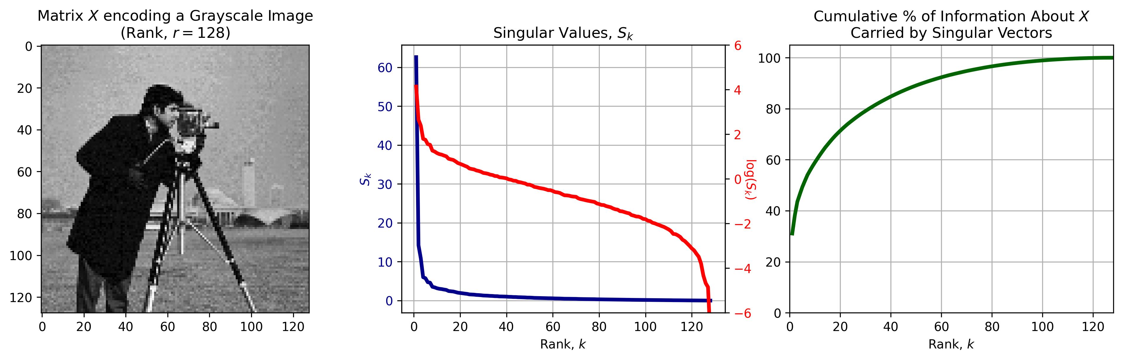
Singular Values for Image Compression — This figure shows a grayscale image, a plot of its singular values (which drop off rapidly), and a plot of the cumulative sum of the singular values' 'energy'. Notice how few singular values are needed to capture most of the image's information.

The rapid decay of singular values is typical for natural images. This means that a vast majority of the image's visual information is contained in the first few singular components. By creating a low-rank approximation $A_{k}$ , we can store the image not as the full $m \times n$ matrix of pixels, but as the three much smaller matrices $U_{k}$ ( $m \times k$ ), $Σ_{k}$ ( $k \times k$ ), and $V_{k}^{T}$ ( $k \times n$ ). For a small $k$ , this results in significant storage savings.

The following reading provides a detailed walkthrough of this process, which will feel very natural given your background in computer science.

The SVD and Image Compression

This document from Brigham Young University's ACME labs provides a hands-on guide to using SVD for image compression, complete with visual examples and problem descriptions that resemble coding assignments.

Please read the sections 'Using the SVD for Data Compression' and 'Image Compression' (pages 4-7). Pay attention to Figure 6.3, which shows how the quality of the image improves as the rank of the approximation increases. Note how color images are handled by applying SVD to each color channel (Red, Green, Blue) separately.

6. How Many Ranks to Keep?

A practical question remains: how do we choose the rank $k$ ? As we saw with image compression, it's a trade-off. A smaller $k$ gives more compression but lower fidelity, while a larger $k$ is more accurate but less compressed.

One popular heuristic is to choose a rank $k$ that preserves a certain percentage (e.g., 90%) of the total "energy" of the matrix. The total energy is defined as the sum of the squares of all singular values.

Fraction of energy preserved = \frac{\sum _{i = 1}^{k} σ _{i}^{2}}{\sum _{i = 1}^{r} σ _{i}^{2}}

We would choose the smallest $k$ that gets this ratio above our desired threshold.

Lecture 49 — SVD Gives the Best Low Rank Approximation (Advanced) | Stanford

This video from a Stanford course explains this 'energy preservation' rule of thumb for choosing the number of dimensions to keep.

Watch the segment from 5:14 to 6:40. This will give you a practical method for deciding on an appropriate rank for your approximation in real-world scenarios.

Conclusion

This lesson concludes our deep dive into Singular Value Decomposition, and it's a fitting finale. The ability to find the best low-rank approximation is arguably one of SVD's most impactful applications in the modern world.

Key Takeaways:

Any matrix can be expressed as a weighted sum of rank-one matrices: $A = \sum σ_{i} u_{i} v_{i}^{T}$ .
The singular values $σ_{i}$ act as importance weights for each rank-one component.
The best rank- $k$ approximation of a matrix $A$ is found by truncating the SVD, keeping only the first $k$ terms of the sum: $A_{k} = U_{k} Σ_{k} V_{k}^{T}$ .
The Eckart-Young Theorem guarantees that this approximation is optimal, minimizing the error among all possible rank- $k$ matrices.
This technique is the basis for powerful applications like data compression, noise reduction, and discovering latent features in data.

Preview of the Next Module:

You have now completed the module on SVD! We've covered its geometric interpretation, its use in determining fundamental matrix properties, calculating the pseudoinverse, and finding optimal low-rank approximations.

In the next module, Applications in Data Analysis, we will see how these concepts come together to solve real-world problems. Our very first topic will be the least squares problem, which is the mathematical engine behind linear regression. We'll see how the pseudoinverse we learned about gives us a direct way to find the best-fit line through a set of data points, a cornerstone of machine learning.

Recommended resources