Hello! Welcome to the final lesson in our "Data Management & Algorithms" module.
In our previous lesson, we explored the world of data warehousing, contrasting OLTP systems built for transactions with OLAP systems designed for analysis. We have now covered the essentials of managing data. This lesson shifts our focus to the second part of this module's title: algorithms. Specifically, we will dive into one of the most fundamental tasks in all of computer science: sorting.
Today's lesson directly addresses the learning outcome: Contrast basic sorting algorithms with divide-and-conquer approaches (Merge Sort, Quick Sort). By the end of this lesson, you will understand the two main strategies for sorting data and be able to identify the key trade-offs between them, especially in terms of performance. This knowledge is crucial as efficient data processing is a prerequisite for nearly every advanced topic in data science and machine learning.
1. The "Divide and Conquer" Strategy
Before we look at specific algorithms, let's first understand a powerful problem-solving paradigm that separates simple sorting methods from more advanced ones: Divide and Conquer.
The idea is simple: instead of tackling a large, complex problem head-on, you break it down into smaller, more manageable subproblems. You solve these subproblems independently and then combine their solutions to solve the original large problem.
To build a strong intuition for this concept, please watch the following short video. It uses a great analogy to explain the core idea.
Divide & Conquer Algorithm In 3 Minutes
This video from Kantan Coding, titled 'Divide & Conquer Algorithm In 3 Minutes', provides a clear and intuitive explanation of this powerful algorithmic strategy.
Watch the first part of the video (00:00 - 01:12). Focus on the three main steps: 1) Divide the problem, 2) Conquer the subproblems, and 3) Combine the results.
Keep this "divide, conquer, combine" framework in mind as we explore the two categories of sorting algorithms.
2. Category 1: Basic Sorting Algorithms
The first category includes algorithms that are straightforward to understand and implement. They generally work by iteratively comparing and swapping elements until the list is sorted. While simple, their performance degrades significantly as the amount of data grows.
The three most common examples are Bubble Sort, Selection Sort, and Insertion Sort.
10 Sorting Algorithms Easily Explained
The video '10 Sorting Algorithms Easily Explained' from Coding with Lewis gives a quick and clear overview of these basic algorithms. It also introduces the concept of Big O notation, which we use to measure an algorithm's efficiency.
Watch the segments covering the basic sorting algorithms (00:00 - 03:08). For each algorithm, focus on its core mechanic: Bubble Sort (00:00 - 01:32): How does it use adjacent swaps to 'bubble' the largest elements to the end? Selection Sort (01:32 - 02:22): What does it 'select' in each pass through the unsorted portion of the array? Insertion Sort (02:22 - 03:08): How does it build the sorted list by 'inserting' elements one by one?
Key Characteristics of Basic Sorts:
- Strategy: They are typically iterative. They process the list element by element, gradually expanding a sorted portion of the array.
- Simplicity: Their logic is easy to follow. Insertion sort, for example, mimics how many people manually sort a hand of playing cards.
- Performance: Their major drawback is their time complexity. For an input of size , they all have an average and worst-case time complexity of . This "quadratic" growth means that if you double the number of items to sort, the time it takes can increase by a factor of four. This makes them impractical for large datasets.
- Space: They are in-place algorithms, meaning they sort the data within the original array without needing significant additional memory. Their space complexity is .
3. Category 2: Divide-and-Conquer Sorting
This second category of algorithms applies the "Divide and Conquer" strategy to achieve much better performance. Instead of iterating through the list, they break it down recursively. The two most famous examples are Merge Sort and Quick Sort.
10 Sorting Algorithms Easily Explained
Let's return to the '10 Sorting Algorithms Easily Explained' video to see how Merge Sort and Quick Sort implement the Divide and Conquer strategy.
Watch the sections on Merge Sort and Quick Sort (03:08 - 05:44). Merge Sort (03:08 - 04:23): Notice how it divides the array down to single elements and then focuses on the 'merge' step to combine them in sorted order. Quick Sort (04:23 - 05:44): Observe the central role of the 'pivot'. The main work happens during the 'partition' step, which rearranges the array around this pivot.
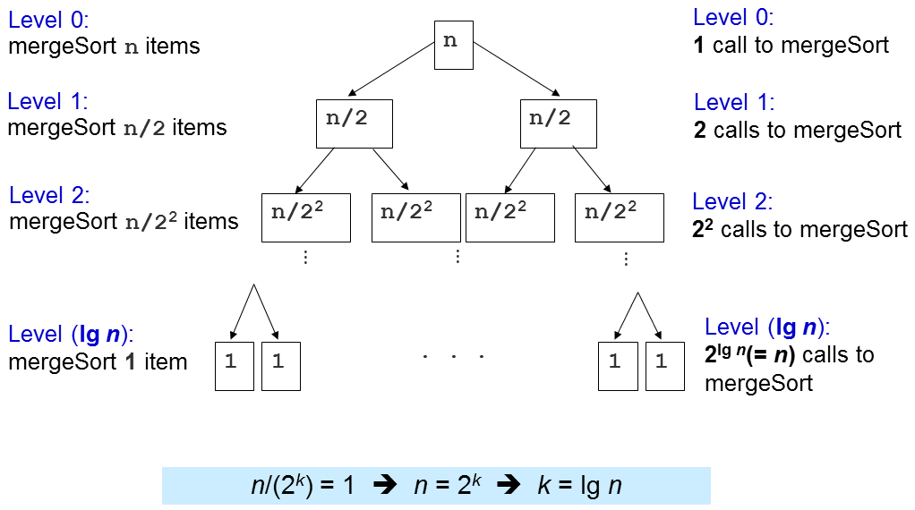
Merge Sort: Divide and Merge
Merge Sort is the classic example of Divide and Conquer.
- Divide: It recursively splits the array in half until it has many sub-arrays of size 1 (which are inherently sorted).
- Conquer & Combine: It then repeatedly merges adjacent sub-arrays, combining them into larger sorted arrays until only one sorted array remains.
Quick Sort: Partition and Recurse
Quick Sort also uses Divide and Conquer, but its approach is different.
- Divide: It selects an element called a pivot and partitions the array. All elements smaller than the pivot are moved to its left, and all elements larger are moved to its right. This partition step is the "conquer" phase.
- Conquer & Combine: It then recursively applies the same process to the sub-arrays on the left and right of the pivot. The "combine" step is trivial because the sorting happens during the partitioning.
4. The Contrast: A Head-to-Head Comparison
The difference between these two categories is not just academic; it has massive practical implications for performance. For your GATE exam, being able to quickly compare them on key metrics is essential.
For a comprehensive overview, the tables in the following resource are an excellent study aid.
Time and Space Complexity of All Sorting Algorithms
The article 'Time and Space Complexity of All Sorting Algorithms' from WsCube Tech provides summary tables that are perfect for quick revision. They allow you to compare algorithms at a glance.
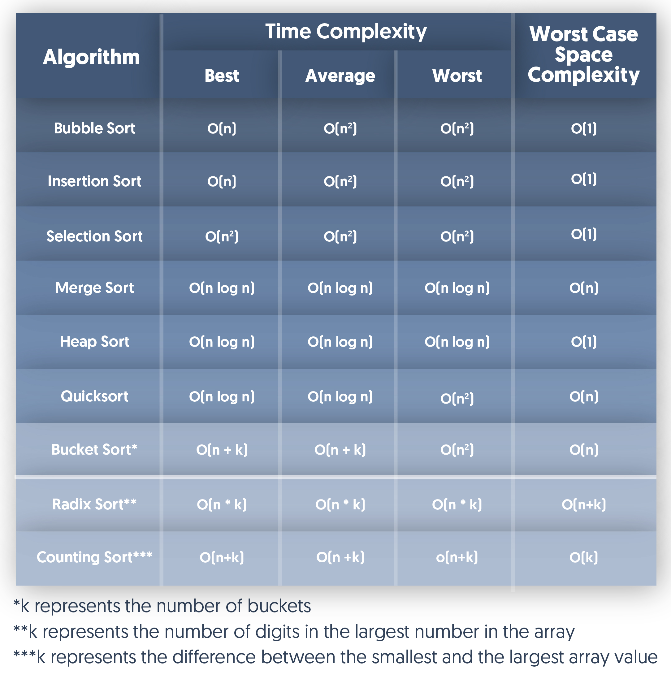
Focus on the two tables: 'Time Complexity of Sorting Algorithms' and 'Space Complexity of Sorting Algorithms'. Notice the stark difference between the O(n²) algorithms and the O(n log n) algorithms.
Here is a summary of the most important contrasts:
| Feature | Basic Sorts (Bubble, Insertion, Selection) | Divide & Conquer (Merge, Quick) |
|---|---|---|
| Core Strategy | Iterative, incremental comparisons. | Recursive, breaking the problem into subproblems. |
| Time Complexity (Average) | — Inefficient for large inputs. | — Highly efficient and scalable. |
| Space Complexity | — In-place, very memory-efficient. | for Merge Sort, for Quick Sort. They require extra memory. |
| Stability | Bubble and Insertion are stable; Selection is not. | Merge Sort is stable; Quick Sort is not. (Stability means equal elements maintain their original relative order). |
| Use Case | Excellent for very small datasets or nearly sorted data (especially Insertion Sort). | The default choice for general-purpose, large-scale sorting. |
This image provides a great visual summary of these complexities.
Conclusion
In this lesson, we have moved from data management to core algorithms, contrasting two fundamental approaches to sorting. You now have the conceptual tools to differentiate between simple, iterative sorting methods and powerful, recursive divide-and-conquer strategies.
Key Takeaways:
- Sorting algorithms are broadly categorized by their underlying strategy.
- Basic Sorts (Bubble, Insertion, Selection) are simple and sort in-place ( space) but are inefficient for large datasets due to their time complexity.
- Divide-and-Conquer Sorts (Merge, Quick) are much faster, with an average time complexity of . This efficiency comes at the cost of extra space ( or ).
- The choice of algorithm depends on the trade-off between simplicity, memory usage, and, most importantly, the size of the data to be sorted.
Preview of the Next Lesson:
This lesson on algorithmic efficiency concludes our module on Data Management & Algorithms. We are now ready to move into the core of modern data science. In our next lesson, we will begin the "Supervised Learning Fundamentals" module, where you will learn how computers can learn from data to make predictions. We will start by asking: What is the difference between regression and classification?