Hello! Welcome to the first lesson in our new module, Supervised Learning Fundamentals.
In our last module, we concluded by looking at how algorithms, like Merge Sort and Quick Sort, can efficiently organize data. Now, we shift from simply organizing data to making predictions from it. This is the core of machine learning.
Today, we will address the learning outcome: Differentiate regression and classification, and describe linear models for both (Linear/Logistic Regression). We'll explore the two primary tasks in supervised learning and introduce the simplest, yet most fundamental, models used to solve them. Understanding this distinction is the first and most crucial step in your machine learning journey.
1. Supervised Learning: Regression vs. Classification
Supervised machine learning is a process where a model learns to make predictions from data that has already been labeled with the correct answers. Think of it like a student studying with an answer key. The goal is to learn the underlying pattern so well that the model can predict the correct answer for new, unseen data.
Within supervised learning, there are two main types of problems: regression and classification. The difference lies entirely in the kind of output you want to predict.
To get a quick and clear overview, let's watch the beginning of the following video.
All Machine Learning algorithms explained in 17 min
The video 'All Machine Learning algorithms explained in 17 min' by Infinite Codes provides a great starting point. It clearly defines supervised learning and breaks down the difference between regression and classification.
Watch the segment from 00:52 to 02:55. As you watch, focus on the examples given for each type of problem: Regression: What kind of value is being predicted (e.g., house price)? Classification: What kind of value is being predicted (e.g., cat or dog)?
As the video explained:
- Regression is used when the target variable is a continuous numerical value. The goal is to predict a quantity.
- Example: Predicting the price of a house, the temperature tomorrow, or a student's score on an exam.
- Classification is used when the target variable is a discrete categorical label. The goal is to predict a class or category.
- Example: Classifying an email as 'spam' or 'not spam', identifying a tumor as 'benign' or 'malignant', or recognizing a handwritten digit.
Now, let's look at the foundational linear model for each of these tasks.
2. Linear Regression: Predicting Continuous Values
Linear Regression is the "hello world" of machine learning models. It's used for regression tasks and is built on a simple premise: the relationship between the input features and the output target can be modeled by a straight line.
The model takes the form of the familiar equation for a line:
Where:
- is the predicted target value (e.g., house price).
- is the input feature (e.g., square footage).
- is the coefficient (or weight), representing the slope of the line. It tells us how much changes for a one-unit change in .
- is the intercept, representing the value of when is zero.
The goal of training a linear regression model is to find the optimal values for and that create the "line of best fit"—the line that minimizes the overall error between its predictions and the actual data points. This error is typically measured using a cost function, most commonly the Mean Squared Error (MSE), which calculates the average of the squared differences between predicted and actual values.
For a quick textual summary and a look at the formulas, please review the following resource.
Linear and Logistic Regression in Machine Learning - EJable
The article 'Linear and Logistic Regression in Machine Learning' from EJable provides a concise written explanation of Linear Regression.
Read the sections titled 'What are Regression and Classification?', 'What is Linear Regression', 'Optimizing the values of our dependent variables', and 'Evaluating Accuracy of Model (Cost Function)'. Focus on understanding the model's equation and the purpose of the cost function (MSE).
3. Logistic Regression: Predicting Categories
Now, what if we want to solve a classification problem? For example, predicting whether a student will pass (1) or fail (0) based on hours studied. It might be tempting to use linear regression, but it quickly falls apart.
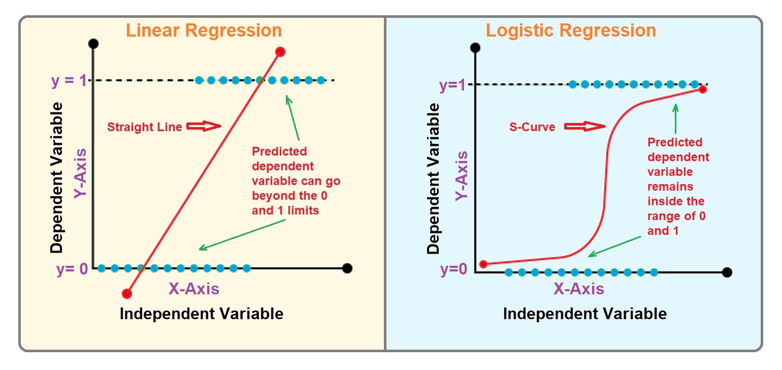
As shown above, a linear regression line can predict values above 1 or below 0, which makes no sense for a pass/fail outcome. We need a model that outputs a probability between 0 and 1. This is where Logistic Regression comes in.
Logistic Regression works in two steps:
- It calculates a linear combination of the input features, just like linear regression: .
- It then feeds this result into a special function called the Sigmoid function, which "squashes" the value into a range between 0 and 1.
The Sigmoid function looks like this:
The output, , can be interpreted as the probability of the positive class (e.g., the probability of passing the exam). We can then use a threshold (typically 0.5) to make a final classification: if the probability is > 0.5, we predict 'Pass'; otherwise, we predict 'Fail'.
Because the output is a probability, the MSE cost function is no longer suitable. Instead, Logistic Regression uses a cost function called Cross-Entropy (or Log Loss). Intuitively, cross-entropy heavily penalizes the model when it makes a confident but incorrect prediction (e.g., predicting a 99% chance of passing for a student who actually failed).
The following video provides an excellent visual explanation of why linear regression is a poor choice for classification and how logistic regression solves the problem.
Logistic Regression (and why it's different from Linear Regression)
The video 'Logistic Regression (and why it's different from Linear Regression)' by Visually Explained gives a fantastic intuition-based walkthrough.
Watch the segments from 00:59 to 06:39. Pay close attention to: Why Linear Regression fails (00:59 - 02:28): Understand the problem of unbounded outputs. The Sigmoid Solution (02:28 - 03:22): See how the S-shaped curve transforms the output into a probability. A New Cost Function (03:22 - 06:39): Grasp the intuition behind why cross-entropy is a better fit for classification than mean squared error.
4. A Head-to-Head Comparison
For the GATE exam, you need to quickly recall the key differences between these two foundational models. Here is a summary table:
| Feature | Linear Regression | Logistic Regression |
|---|---|---|
| Problem Type | Regression | Classification (primarily binary) |
| Output | Continuous numerical value | Probability (a value between 0 and 1) |
| Model | Fits a straight line to data | Fits an 'S'-shaped curve (Sigmoid) |
| Equation | ||
| Cost Function | Mean Squared Error (MSE) | Cross-Entropy (Log Loss) |
| Goal | Minimize the distance between predicted and actual values. | Maximize the probability of the correct class. |
A quick note on naming: It's often confusing that "Logistic Regression" has "regression" in its name when it's used for classification. This is largely for historical reasons. The model regresses on the log-odds of the outcome, but its practical application and purpose in machine learning is classification.
Conclusion
Congratulations on completing your first lesson in supervised learning! You've learned to distinguish between the two most fundamental tasks in the field and have been introduced to the benchmark linear model for each.
Key Takeaways:
- Supervised learning involves training a model on labeled data to make predictions.
- Regression predicts continuous, numerical outcomes (e.g., price), while Classification predicts discrete, categorical outcomes (e.g., spam/not spam).
- Linear Regression is the go-to model for regression tasks. It fits a straight line and aims to minimize the Mean Squared Error (MSE).
- Logistic Regression is the foundational model for binary classification. It uses the Sigmoid function to output a probability and minimizes the Cross-Entropy loss.
Preview of the Next Lesson:
Linear models are powerful, but many real-world relationships aren't straight lines. In the next lesson, we will explore some popular and intuitive non-linear classifiers, including k-Nearest Neighbors (k-NN), Naive Bayes, Support Vector Machines (SVMs), and Decision Trees.