Intuition Behind Non-Linear Classifiers

1. An Overview of Non-Linear Classifiers

While logistic regression draws a single straight line (or a hyperplane in higher dimensions) to separate classes, many real-world datasets aren't so cleanly separable. Non-linear classifiers use different strategies to create more flexible decision boundaries.

We'll take a quick tour of four of the most important ones. The following video provides a rapid, high-level introduction to all of them. We will watch it in segments as we discuss each algorithm.

2. K-Nearest Neighbors (k-NN): The "Neighborhood Watch"

The core idea of k-NN is simple and intuitive: a data point is classified based on the class of its closest neighbors.

Imagine plotting all your data on a graph. To classify a new, unknown point, you find the 'k' points from your training data that are closest to it. The new point is then assigned the class that is most common among those 'k' neighbors (a majority vote).

Let's see a quick explanation.

Key Intuition:

• Mechanism: "Tell me who your friends are, and I'll tell you who you are." It's a simple voting system based on proximity.
• The 'k' value: This is a hyperparameter you must choose.
  • A small k (e.g., 1) makes the model highly sensitive to noise and can lead to overfitting.
  • A large k can oversmooth the decision boundary and lead to underfitting.
• Lazy Learner: k-NN is called a "lazy" algorithm because it doesn't build a model during training. It simply stores the entire training dataset. The real work (calculating distances) happens only when a new prediction is requested, which can make it slow for large datasets.

3. Naive Bayes: Leveraging Probability

The Naive Bayes classifier is based on Bayes' Theorem, which you may recall from your probability studies. It calculates the probability that a data point belongs to a particular class, given its features.

The "naive" part of the name comes from a strong, and often unrealistic, assumption: it assumes that all features are independent of each other. For example, in a spam filter, it assumes the probability of the word "free" appearing is completely independent of the probability of the word "money" appearing. While this isn't true, the algorithm is surprisingly effective and computationally very fast.

Key Intuition:

• Mechanism: Uses Bayes' theorem to find $P(\text{Class}|\text{Features})$. It chooses the class with the highest probability.
• The "Naive" Assumption: The independence of features makes the calculations extremely efficient. This is the model's defining characteristic.
• Use Case: It excels in text classification problems like spam detection and sentiment analysis.

4. Support Vector Machine (SVM): Finding the Widest Street

The goal of a Support Vector Machine is to find the optimal decision boundary that best separates the classes. It doesn't just find any boundary; it finds the one that is as far away as possible from the nearest data points of each class. This gap is called the margin, and the SVM tries to maximize it.

The data points that lie on the edge of this margin are called support vectors—they are the critical points that "support" the decision boundary.

Key Intuition:

• Mechanism: Finds a hyperplane (a line in 2D, a plane in 3D, etc.) that creates the largest possible margin between classes. This makes the model more robust to new data.
• Support Vectors: These are the most important data points in the training set, as they define the margin. The model is efficient because it only depends on these points.
• The Kernel Trick: For data that is not linearly separable, SVMs can use a "kernel trick" to project the data into a higher dimension where a linear boundary can be found. This is how SVMs powerfully handle non-linear problems without you having to manually create new features.

5. Decision Trees: A Flowchart of Questions

A Decision Tree is perhaps the most intuitive classifier. It works like a flowchart, where each internal node represents a "test" on a feature (e.g., "Is age < 50?"), each branch represents the outcome of the test (Yes/No), and each leaf node represents a class label.

The algorithm learns a sequence of questions to ask that best split the data into "pure" groups (i.e., groups containing members of only one class).

Key Intuition:

• Mechanism: Splits the data recursively based on feature values. It's easy to visualize and interpret.
• Purity: The goal at each split is to increase the purity of the resulting nodes. A perfectly pure node contains data points from only one class.
• Overfitting: A major risk with decision trees is that they can grow too deep, learning the training data perfectly but failing to generalize to new data. Techniques like pruning (limiting the tree's depth) are used to combat this.

6. A Quick Comparison: Pros and Cons

For the GATE exam, knowing the relative strengths and weaknesses of these models is essential for answering "which algorithm is best for...?" type questions. The following table provides a fantastic summary.

Now, let's look at a head-to-head comparison.

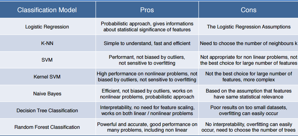
Let's distill the key trade-offs:

• Decision Tree: Pro: Very easy to interpret and explain. Con: Prone to overfitting.
• k-NN: Pro: Simple to understand and implement. Con: Computationally expensive for large datasets because it needs to compare a new point to all existing points.
• SVM: Pro: Very effective in high-dimensional spaces and robust against overfitting. Con: Can be computationally intensive and less interpretable (the "kernel trick" can feel like a black box).
• Naive Bayes: Pro: Extremely fast and performs well with high-dimensional data like text. Con: The "naive" assumption of feature independence is often violated in reality.

Conclusion

In this lesson, you've gained a high-level intuition for four fundamental non-linear classifiers. You've moved beyond the simple linear world and now have a set of powerful and flexible tools in your conceptual toolkit.

Key Takeaways:

• k-Nearest Neighbors (k-NN) classifies based on majority vote of the nearest data points.
• Naive Bayes uses probability (Bayes' theorem) and a strong "independence" assumption to classify data quickly.
• Support Vector Machines (SVM) aim to find the decision boundary with the maximum possible margin for robustness.
• Decision Trees create a flowchart of rules that are easy to interpret but can be prone to overfitting.

Preview of the Next Lesson:
We've now seen several different models. But how do we choose the best one? And how do we tune them (like choosing 'k' in k-NN) to perform well on new, unseen data? The next lesson, "Explain the bias-variance trade-off and the role of cross-validation in model evaluation," will give us the framework to answer these critical questions.