Welcome to the third lesson in our "Data Management & Algorithms" module.
In our last lesson, we focused on designing efficient and reliable databases using normalization and indexing. We learned that these techniques are crucial for systems that handle day-to-day operations, which we briefly identified as Online Transaction Processing (OLTP) systems.
Today, we will explore the other side of the data universe. While OLTP systems are built to run the business, a different kind of system is needed to analyze the business. This lesson directly addresses the learning outcome: Contrast OLTP databases with data warehousing concepts (schemas, OLAP). We will explore what happens when data is moved from operational databases into a specialized environment—a data warehouse—built for analysis and decision-making.
1. Two Worlds of Data: Transactional vs. Analytical
Imagine an e-commerce platform. When you buy a product, the system instantly records the sale, updates the inventory, and confirms your payment. This is a transaction. The database supporting this must be fast, accurate, and always available for these small, frequent updates. This is the world of OLTP (Online Transaction Processing).
Now, imagine the company's CEO wants to know which products were most profitable in the last quarter, broken down by region and customer demographic. This requires looking at months of historical sales data, aggregating it, and slicing it in different ways. This is analysis. The system for this must be optimized for complex queries over vast amounts of data. This is the world of OLAP (Online Analytical Processing).
The following video gives an excellent real-world analogy to frame the difference between these two fundamental concepts.
Lec -7: OLAP vs OLTP | Difference between OLAP vs OLTP with Real Life Examples
This video from Gate Smashers, a channel popular for GATE preparation, uses a simple analogy to introduce OLTP and OLAP. It will help you build a strong intuition for their different purposes.
Watch the video from the beginning until 06:17. As you watch, focus on how the two systems differ in their: Purpose: User-facing transactions vs. business-facing analysis (00:00 - 01:57). Data: Current, operational data vs. historical, multi-dimensional data (01:57 - 03:40). Queries & Users: Simple queries by front-line staff vs. complex queries by analysts and executives (03:40 - 05:07). Response Time & Updates: Fast, real-time responses vs. slower, periodic updates (05:07 - 06:17).
Key Differences at a Glance
To summarize the distinctions for your quick review, the table below is a crucial resource. It lays out the core contrasts between OLTP and OLAP systems side-by-side.
Difference Between OLAP and OLTP in Databases
The article 'Difference Between OLAP and OLTP in Databases' from GeeksforGeeks provides a concise but comprehensive comparison. The summary table is particularly useful for exam revision.
Focus on the main comparison table under the heading 'Difference Between OLAP and OLTP'. This table efficiently summarizes everything you need to know to contrast the two systems.
Here is another excellent visual summary of the key differences:

2. The Heart of OLAP: Data Warehouses and Schemas
OLAP systems don't run on the same databases as OLTP systems. Instead, they use a Data Warehouse. A data warehouse is a large, central repository of data that is consolidated from one or more disparate sources (like OLTP databases). Its entire structure is optimized for analysis, not transactions.
In our last lesson, we saw that OLTP systems use normalized tables (e.g., in 3NF) to reduce redundancy and ensure data integrity during frequent writes. This structure is inefficient for the complex, read-heavy queries of OLAP.
Instead, data warehouses use denormalized structures called schemas. The goal is to arrange data to make querying for analysis intuitive and fast, even if it means introducing some data redundancy. The basic building blocks of these schemas are:
- Fact Tables: These tables contain the quantitative data or "facts" you want to measure, like
SalesAmount,QuantitySold, orProfit. They are typically very large. - Dimension Tables: These tables contain the descriptive attributes that provide context to the facts, such as
ProductDetails,CustomerInfo,StoreLocation, orDate. They answer the "who, what, where, when" questions about the facts.
The way these tables are arranged defines the schema. The two most important schemas for you to know are the Star Schema and the Snowflake Schema.
To understand these concepts visually, watch the following explanation.
What is STAR schema | Star vs Snowflake Schema | Fact vs Dimension Table
This video from codebasics provides one of the clearest explanations of fact/dimension tables and how they form Star and Snowflake schemas. It uses a simple grocery store example to make the concepts very easy to grasp.
Watch the section from 03:17 to 06:34. Pay close attention to: Fact vs. Dimension Tables (03:17 - 04:45): Understand what each table type holds and how they relate to form the Star Schema. Snowflake Schema (04:45 - 06:34): See how this schema is just an extension of the Star Schema where the dimension tables are themselves normalized.
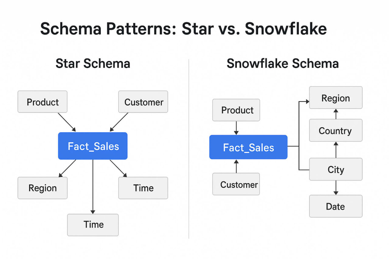
Visualizing Star vs. Snowflake Schemas
The names "Star" and "Snowflake" come from the visual layout of the tables.
- Star Schema: A central fact table is directly connected to several denormalized dimension tables. It looks like a star. This simple structure requires fewer joins, making queries faster.
- Snowflake Schema: This is an extension of the star schema where the dimension tables are normalized into multiple related tables. This reduces redundancy and can make the model easier to maintain, but it requires more joins, which can slow down queries.
The image below clearly illustrates this structural difference.
For a final review, the article below gives a great text-based summary of when and why you might choose one schema over another.
Data Warehouse Schemas Explained: Star, Snowflake, Galaxy
The article 'Data Warehouse Schemas Explained' clearly defines the different schemas and provides guidance on their use cases.
Quickly read the following sections to solidify your understanding: 'STAR Schema': Reinforces the structure and benefits (performance). 'Snowflake Schema': Reinforces its structure and benefits (less redundancy, data integrity). 'Conclusion': Provides a practical guideline on when to choose each schema.
Conclusion
In this lesson, we have contrasted the two primary paradigms of database systems. You now understand the fundamental differences between a system designed to handle daily transactions and one designed to derive business intelligence from historical data.
Key Takeaways:
- OLTP (Online Transaction Processing) systems are for running day-to-day business operations. They use normalized databases, handle simple read/write queries on current data, and are optimized for speed and consistency.
- OLAP (Online Analytical Processing) systems are for analyzing the business to support decision-making. They use data warehouses with specialized schemas, handle complex, read-only queries on large historical datasets, and are optimized for analytical performance.
- Data warehouse schemas organize data for analysis. The most common are:
- Star Schema: A central fact table with denormalized dimension tables. It is simple and fast.
- Snowflake Schema: A star schema with normalized dimension tables. It saves space but can be slower due to more complex joins.
Preview of the Next Lesson:
We will now shift gears from data management to algorithms. In our next lesson, we will dive into the world of sorting data efficiently. We will contrast basic sorting algorithms with more advanced divide-and-conquer approaches like Merge Sort and Quick Sort, which are fundamental concepts in computer science and data processing.