Optimizing with Derivatives: Maxima and Minima

1. The Goal: Finding Peaks and Valleys

In optimization, we are interested in finding the extrema of a function—its maximum and minimum values.

• A local maximum is a point that is higher than all its immediate neighbors. It's a "peak" in the local landscape.
• A local minimum is a point that is lower than all its immediate neighbors. It's a "valley" in the local landscape.

At these peaks and valleys (for a smooth, differentiable function), the tangent to the curve is perfectly horizontal. This means the slope, or the first derivative, is zero. We call these points stationary points or critical points.

2. Step 1: Finding Stationary Points

The first step in any optimization problem is to find the candidates for maxima and minima. As we've just discussed, this means finding the points where the first derivative is zero.

The process is straightforward:

1. Given a function $f(x)$, find its first derivative, $f^{\prime }(x)$.
2. Set the derivative to zero: $f^{\prime }(x)=0$.
3. Solve this equation for $x$. The solutions are the x-coordinates of your stationary points.

To see this process in action, let's watch a short video that walks through an example.

Once we have these stationary points, we need a way to determine whether each one is a maximum, a minimum, or neither. This is where the derivative tests come in.

3. Step 2: Classifying Stationary Points

There are two primary methods for classifying stationary points.

Method A: The Second Derivative Test

The second derivative, $f^{\prime \prime }(x)$, tells us about the concavity of the function. It measures the rate of change of the slope.

• If $f^{\prime \prime }(x)>0$, the slope is increasing. The curve is shaped like a 'U' (concave up).
• If $f^{\prime \prime }(x)<0$, the slope is decreasing. The curve is shaped like an 'n' (concave down).

This gives us a very direct test. For a stationary point $c$ (where $f^{\prime }(c)=0$):

1. If $f^{\prime \prime }(c)>0$, the point is a local minimum. (Concave up, like a valley)
2. If $f^{\prime \prime }(c)<0$, the point is a local maximum. (Concave down, like a peak)
3. If $f^{\prime \prime }(c)=0$, the test is inconclusive. We can't draw a conclusion from the second derivative alone and must use the first derivative test.

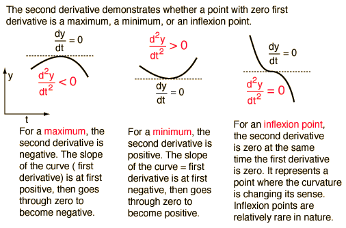
Let's continue with the same video to see a highly intuitive explanation and a worked example of this test.

Method B: The First Derivative Test

This test is more general and works even when the second derivative test is inconclusive. Here, we analyze the sign of the first derivative, $f^{\prime }(x)$, on either side of the stationary point $c$.

1. If $f^{\prime }(x)$ changes from positive to negative at $c$, the function goes from increasing to decreasing. This means $c$ is a local maximum.
2. If $f^{\prime }(x)$ changes from negative to positive at $c$, the function goes from decreasing to increasing. This means $c$ is a local minimum.
3. If $f^{\prime }(x)$ does not change sign at $c$ (e.g., positive on both sides), then $c$ is neither a maximum nor a minimum. It is likely a point of inflection.

For the GATE exam, you need fast methods. The "wavy curve method" is a quick way to analyze the sign of the derivative, especially for polynomial functions.

4. Summary of the Tests

To consolidate these rules, it's helpful to have a concise reference. The following document provides a clear, formal summary of both tests.

This resource also includes several worked examples that you can review later if you wish to see more applications of these tests.

Conclusion

In this lesson, we've covered the fundamental calculus techniques for finding and classifying the maxima and minima of single-variable functions. This process of optimization is central to training machine learning models, where the "function" is a cost function and the "minimum" represents the best possible model parameters.

Key Takeaways:

• Stationary points are candidates for maxima or minima, found by setting the first derivative to zero ($f^{\prime }(x)=0$).
• The Second Derivative Test is often the fastest way to classify a stationary point $c$:
  • $f^{\prime \prime }(c)>0⟹$ local minimum.
  • $f^{\prime \prime }(c)<0⟹$ local maximum.
  • $f^{\prime \prime }(c)=0⟹$ inconclusive.
• The First Derivative Test is a more general method. It checks the sign of $f^{\prime }(x)$ around the stationary point $c$:
  • Sign change + to - $⟹$ local maximum.
  • Sign change - to + $⟹$ local minimum.
  • No sign change $⟹$ neither (e.g., point of inflection).

Preview of the Next Lesson:
We will conclude our tour of calculus by looking at Taylor series. While today's topic was about finding exact maxima and minima, Taylor series are about approximating a complex function with a simpler polynomial around a specific point. This is another powerful tool that relies on derivatives to understand a function's local behavior.