Taylor Series for Function Approximation

Hello! Welcome to the final lesson in our "Essential Mathematical Foundations" module.

In our last lesson, we explored how to use first and second derivatives to find and classify the maxima and minima of functions. We saw that derivatives give us powerful insights into a function's local behavior, like its slope and curvature. Today, we'll use that same idea—derivatives describing local behavior—for a different but equally important purpose: function approximation.

This lesson addresses the learning outcome: Describe the purpose of Taylor series for function approximation. We'll discover how we can use derivatives at a single point to build a simple polynomial that mimics a much more complex function. This concept is fundamental in many areas of science, engineering, and machine learning, often used to make difficult problems computationally manageable.

1. The Core Idea: Why Approximate?

Imagine your calculator needs to compute sin(0.7) or e^2.3. These are not simple arithmetic operations. How can a machine that only excels at addition, subtraction, multiplication, and division compute these values so quickly?

The answer is approximation. Instead of dealing with the "true" complex function, we can create a simple polynomial (e.g., $c_{0} + c_{1} x + c_{2} x^{2}$ ) that behaves almost identically to the real function around the value we care about. Taylor series provide a systematic way to construct these polynomial approximations.

Let's start with a short video that gives a fantastic visual intuition for this process.

Taylor Series - Explained

This video from DataMListic beautifully illustrates the core concept of Taylor series. It shows how a complex function can be progressively approximated by matching its properties at a single point.

Watch the video from the beginning until 03:41. As you watch, focus on how the approximation improves with each step: 0th Order (Constant): Matching the function's value (height). 1st Order (Linear): Matching the first derivative (slope). 2nd Order (Quadratic): Matching the second derivative (curvature).

As you saw, the magic of Taylor series is that we can build a remarkably good approximation of a function in a local neighborhood using only information from a single point—its value and the values of its successive derivatives.

2. Building the Approximation: The Taylor Formula

The video gave us the intuition. Now, let's formalize it. How do we find the exact coefficients for our approximating polynomial? The key is to force the polynomial's derivatives to match the function's derivatives at our chosen point of expansion, which we'll call $a$ .

Let's say we want to approximate a function $f (x)$ near $x = a$ with a polynomial $P (x)$ .

To match the value, we set $P (a) = f (a)$ .
To match the slope, we set $P^{'} (a) = f^{'} (a)$ .
To match the curvature, we set $P^{''} (a) = f^{''} (a)$ .
...and so on for all higher derivatives.

The following video walks through this derivation to arrive at the general formula for a Taylor series.

Intro to Taylor Series: Approximations on Steroids

Dr. Trefor Bazett provides a clear, step-by-step derivation of the coefficients of the Taylor polynomial. This will show you exactly where the formula comes from.

Watch the segment from 03:20 to 10:10. Focus on: The process of matching the value, first derivative, and second derivative of e^x at x=0 to find the coefficients for its quadratic approximation. How taking the n-th derivative of a term c_n * x^n leads to the n! (n-factorial) term. The final, generalized formula for the coefficients and the distinction between a Taylor series (around any point 'a') and a Maclaurin series (around a=0).

This process gives us the Taylor series expansion of a function $f (x)$ around a point $a$ :

f (x) \approx n = 0 \sum \infty \frac{f ^{(n)} ( a )}{n !} (x - a)^{n}

Where:

$f^{(n)} (a)$ is the n-th derivative of $f$ evaluated at the point $a$ .
$n!$ is the factorial of n.
When $a = 0$ , this is called a Maclaurin series.

A finite number of terms from this series is called a Taylor polynomial. For example, the second-order Taylor polynomial for $f (x)$ around $a$ is:

P_{2} (x) = f (a) + f^{'} (a) (x - a) + \frac{f ^{''} ( a )}{2 !} (x - a)^{2}

3. Reading for Reinforcement and Reference

To consolidate your understanding, let's turn to a well-written article that walks through the same logic with a different example, cos(x). This will help reinforce the pattern and the purpose of each term.

Taylor series - 3Blue1Brown

The following article from 3Blue1Brown explains the same concepts we've just seen, but with a focus on approximating cos(x). It's a great way to review the material and see it in a textual format.

Please read the following sections: 'Approximating cos(x)': Follow the step-by-step logic for finding the quadratic approximation by matching the value, derivative, and second derivative. 'Better Approximations': See how adding a fourth-degree term improves the fit. 'Other Functions' and 'A meaningful example': Review the general formula and see the Taylor series for e^x, one of the most famous examples. Focus on how each coefficient is chosen to match a specific derivative.

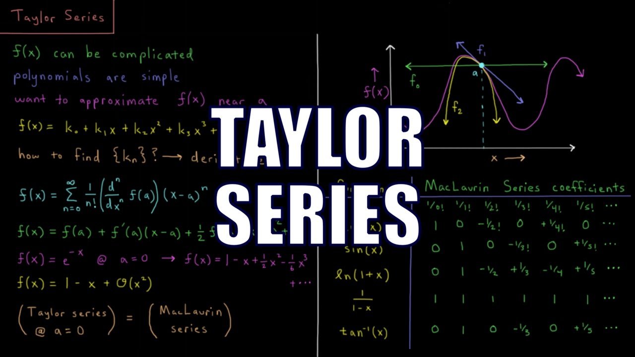
For quick reference, which is invaluable for exam preparation, the following image summarizes the Taylor series formula and provides the Maclaurin series for several common functions.

Taylor Series Overview with Maclaurin Coefficients — A handy cheat sheet summarizing the Taylor series formula, its graphical intuition, and the Maclaurin series for several important functions.

Conclusion

In this lesson, we demystified Taylor series, seeing them as a systematic tool for approximating complex functions with simpler polynomials. This is a cornerstone of numerical methods and optimization theory.

Key Takeaways:

Purpose: Taylor series allow us to approximate a complex, non-polynomial function (like sin(x) or e^x) with a simple polynomial around a specific point.
Mechanism: The approximation is built by constructing a polynomial whose value and derivatives (slope, curvature, etc.) match those of the original function at the point of expansion (a).
Formula: The coefficient of the $(x - a)^{n}$ term is determined by the function's n-th derivative at a, divided by $n!$ .
Trade-off: More terms in the polynomial lead to a better approximation over a wider range, but at the cost of increased complexity.
Application in ML: Taylor series are used to approximate objective functions in optimization algorithms. For example, Newton's method in optimization is derived from a second-order Taylor approximation of a function.

This lesson concludes our module on Essential Mathematical Foundations. We have rapidly surveyed key ideas from linear algebra (eigenvectors, decompositions) and calculus (optimization, approximation) that form the mathematical bedrock of many data science and machine learning techniques.

Preview of the Next Lesson:
We will now shift gears and begin a new module: Data Management & Algorithms. Our first lesson will cover the fundamentals of how data is stored and managed in modern systems, starting with the core concepts of the relational model (ER diagrams, tables, keys) and the language used to query it, SQL.

Recommended resources

1. The Core Idea: Why Approximate?

2. Building the Approximation: The Taylor Formula

3. Reading for Reinforcement and Reference

Conclusion