Stochastic Anti-Aliasing

The Problem: One Sample Isn't Enough

As we've discussed, the core of our ray tracer so far involves sending a single ray through the center of each pixel. This is a form of point sampling—we're trying to determine the color of a square area (the pixel) by checking the color at just one single point within it.

This is a poor approximation. If a pixel straddles the edge of an object, that single sample will either hit the object or miss it entirely. The result is a binary, all-or-nothing decision that creates the harsh, staircase-like edges you see in your renders.

To solve this, we need to gather more information about the area that the pixel covers.

The solution, as the article suggests, is to average the results from multiple samples. Instead of one ray per pixel, we'll cast many. This is a form of Monte Carlo integration, where we use random sampling to approximate a definite integral—in this case, the integral of light coming through the pixel's area.

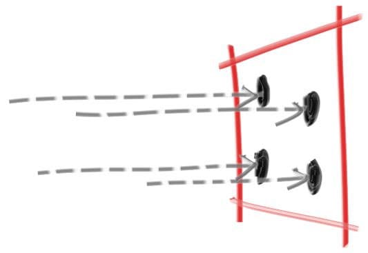
The Antialiasing Algorithm

The logic for multi-sample antialiasing is a straightforward extension of our current rendering loop:

1. For each pixel in the image:
2. Initialize an accumulator for the color (e.g., vec3 pixel_color(0, 0, 0)).
3. Loop a fixed number of times (e.g., 100 times). Let's call this samples_per_pixel.
   a. For the current sample, calculate a randomly jittered position within the current pixel.
   b. Generate a ray that passes from the camera through this new jittered point.
   c. Call ray_color() to get the color for this one ray.
   d. Add the resulting color to your pixel_color accumulator.
4. After the inner loop finishes, divide the accumulated pixel_color by samples_per_pixel to get the average color.
5. Write this final average color to your image file.

Implementing Multi-Sample Antialiasing

Let's translate this algorithm into C++. We'll primarily be modifying the main render loop in your main.cpp file. The canonical guide, Ray Tracing in One Weekend, provides a very clean implementation.

Based on this guide, here are the changes you'll need to make in your main.cpp:

1. Add a constant for the number of samples. At the top of your main function, define how many samples you want per pixel. 100 is a good starting point for a high-quality result.

   // Image
   const auto aspect_ratio = 16.0 / 9.0;
   const int image_width = 400;
   const int image_height = static_cast<int>(image_width / aspect_ratio);
   const int samples_per_pixel = 100; // New!
   

2. Modify your main render loop. You need to wrap your existing ray generation logic inside a new loop that runs samples_per_pixel times, accumulating the color.

   // Render
   std::cout << "P3\n" << image_width << ' ' << image_height << "\n255\n";
   
   for (int j = image_height - 1; j >= 0; --j) {
       std::cerr << "\rScanlines remaining: " << j << ' ' << std::flush;
       for (int i = 0; i < image_width; ++i) {
           color pixel_color(0, 0, 0); // Initialize accumulator
           for (int s = 0; s < samples_per_pixel; ++s) {
               // Generate a randomly jittered ray for this pixel
               auto u = (i + random_double()) / (image_width - 1);
               auto v = (j + random_double()) / (image_height - 1);
               ray r = cam.get_ray(u, v);
               // Add this sample's color to the accumulator
               pixel_color += ray_color(r, world); 
           }
           // Write the final, averaged color
           write_color(std::cout, pixel_color, samples_per_pixel);
       }
   }
   

3. Update your write_color function. Your write_color function previously just wrote the color it was given. Now, it needs to perform the division by samples_per_pixel to get the average.

   // In your color utility header (or wherever write_color is defined)
   void write_color(std::ostream &out, color pixel_color, int samples_per_pixel) {
       auto r = pixel_color.x();
       auto g = pixel_color.y();
       auto b = pixel_color.z();
   
       // Divide the color by the number of samples.
       auto scale = 1.0 / samples_per_pixel;
       r *= scale;
       g *= scale;
       b *= scale;
   
       // Write the translated [0,255] value of each color component.
       out << static_cast<int>(256 * clamp(r, 0.0, 0.999)) << ' '
           << static_cast<int>(256 * clamp(g, 0.0, 0.999)) << ' '
           << static_cast<int>(256 * clamp(b, 0.0, 0.999)) << '\n';
   }
   

   Don't forget to update the function signature in its declaration as well.

After making these changes, compile and run your program. You'll immediately notice two things: the image quality is dramatically better, and the render time is significantly longer.

The Trade-off: Quality vs. Performance

This trade-off is fundamental to ray tracing and especially relevant in a VFX production environment. More samples give you a cleaner image (less noise), but at the cost of longer render times. Finding the right balance is a constant challenge.

A Glimpse of Production Techniques: Progressive Rendering

Our current implementation is what's known as a "bucket" renderer: it completely finishes one pixel (calculates all its samples) before moving to the next.

Many modern renderers used in DCC tools like Houdini or Maya use a different approach for their interactive preview windows (often called IPR for "Interactive Photorealistic Rendering"). They use progressive rendering.

The idea is to get a noisy, full-image preview very quickly, and then progressively refine it over time. This is achieved by:

1. Creating an "accumulation buffer" in memory to store the running total color for each pixel.
2. In the first pass, trace one random ray for every pixel and add the result to the buffer. Display the buffer's current state. The image is very noisy.
3. In the second pass, trace another random ray for every pixel, add it to the buffer, and display the average of the two samples. The noise is reduced.
4. Repeat this process. The image converges toward a clean result over time. If the camera moves, the buffer is cleared and the process restarts.

This provides immediate visual feedback, which is invaluable for artists.

While we won't implement a full progressive system right now, it's crucial to understand this concept as it directly relates to the tools you use in your work. Our multi-sample approach is computationally identical; it just organizes the work differently (pixel by pixel instead of frame by frame).

Conclusion

Congratulations! You've implemented one of the most important techniques for improving the visual quality of a ray tracer. The smooth edges on your objects are a direct result of applying a powerful idea from statistics—Monte Carlo sampling—to a graphics problem.

Key Takeaways:

• Aliasing ("jaggies") is caused by under-sampling a pixel's area.
• Multi-sample antialiasing (MSAA) solves this by tracing multiple, randomly jittered rays per pixel and averaging their colors.
• The implementation requires adding a new loop inside your main render loop to accumulate color samples.
• There is a direct, linear trade-off between the number of samples per pixel and the total render time.
• Progressive rendering is a related technique used in production renderers to provide fast, interactive feedback that refines over time.

Next Steps

Now that you've mastered adding randomness to your primary rays for antialiasing, you're ready to apply the same concept to another fundamental camera effect: Depth of Field. In the next lesson, we will simulate a camera's aperture to create realistic focus blur, allowing some parts of your scene to be sharp while others are elegantly blurred. You'll find that the core idea of jittering rays is surprisingly similar to what we've done today.