Hello! Welcome back to our ray tracing journey.
In the last lesson, you successfully created a "world" of objects and rendered your first scene containing more than one shape. This was a huge step, moving us from isolated geometric tests to a scalable scene rendering system.
If you look closely at the image you generated, especially around the edges of the sphere, you'll notice a distinct "stair-step" or jagged effect. This artifact is a classic problem in computer graphics called aliasing.
Today's lesson is dedicated to understanding exactly why this happens. We won't be writing code to fix it just yet; instead, we'll build a solid conceptual foundation for the problem. Understanding the cause is the first step toward implementing an effective solution, a crucial skill for producing the high-quality, realistic images you see from production renderers like Arnold or Karma.
Our goal for this lesson is to explain the cause of aliasing (jaggies) in computer-generated images.
What is Aliasing? A Visual Definition
At its heart, aliasing is the name for artifacts that appear in a digital signal when it's sampled improperly. In computer graphics, the most common and obvious form of aliasing is the "jaggies" we see on the edges of rendered objects.
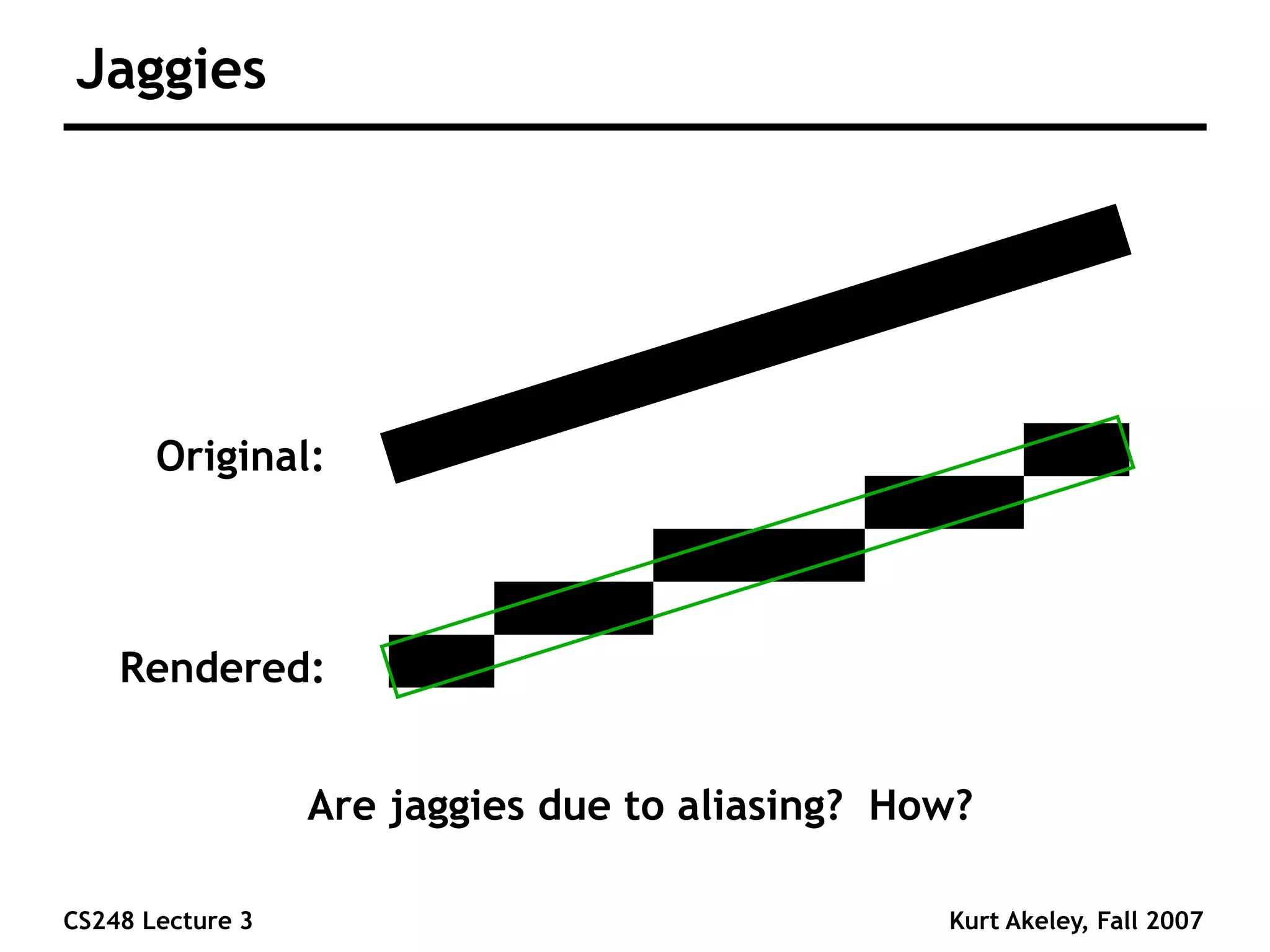
This happens because we are trying to represent a continuous, smooth world on a discrete, finite grid of pixels. The core of the problem lies in how we decide the color of each individual pixel.
Let's watch a short video clip that shows this effect in a 3D scene and introduces the concept of sampling.
Intro to Graphics 21 - Sampling
This clip from Cem Yuksel's 'Intro to Graphics' series provides a clear visual comparison between an aliased and an anti-aliased image, setting the stage for why one looks better than the other.
Watch from 16:36 to 18:15. Pay attention to the comparison between the 'aliased' image with jagged edges and the 'anti-aliased' image with smoother edges, even at the same low resolution.
The Root Cause: Under-sampling a Continuous Function
So, why do these jaggies appear? It's because our ray tracer is taking a shortcut.
For each pixel in our final image, our program currently sends out a single ray through the center of that pixel. The color returned by that one ray becomes the color for the entire pixel square.
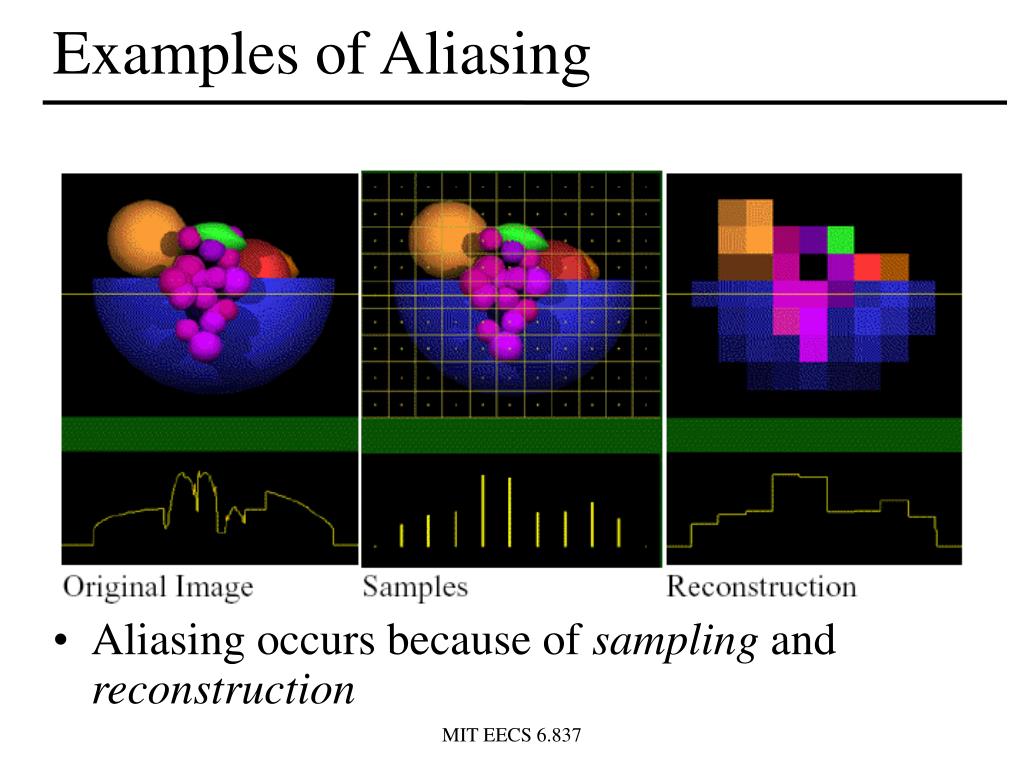
Consider a pixel where a geometric edge passes right through it.
- If our single sample ray happens to hit the object, the entire pixel is colored with the object's color.
- If our single sample ray happens to miss the object, the entire pixel is colored with the background color.
There is no in-between. The pixel is either 100% object or 100% background. As we move from one pixel to the next along an edge, the color can jump abruptly, creating the jagged line.
The "correct" color for that pixel should actually be a blend—an average of all the colors within the pixel's area. To understand this more formally, let's explore a great article on the topic.
The article 'Aliasing in computer graphics' provides a fantastic explanation. We'll start by clarifying a key distinction it makes between 'sampling' and 'quantization'.
Please read the section titled 'Sampling vs quantization'. This will clarify that aliasing comes from the act of sampling (choosing where to measure) and not from quantization (representing the measured color with finite bits).
As the article states, aliasing arises from sampling. Our single-ray-per-pixel strategy is a form of point sampling, and it's a poor approximation of the true color information within the pixel's boundary.
A Signal Processing Perspective
Your computer science background gives us a powerful lens through which to view this problem: digital signal processing (DSP). In DSP, aliasing occurs when a signal is sampled at a rate too low to capture its details.
- The Continuous Signal: Think of the 2D image projected onto your virtual camera plane as a continuous signal. It's defined everywhere, not just at pixel centers.
- High-Frequency Content: A sharp edge, like the silhouette of our sphere, represents a very sudden change in this signal—from background color to object color. In signal processing terms, sudden changes are high-frequency content. A perfectly sharp edge is effectively a step function, which contains infinite frequencies.
- The Sampling Rate: Our pixel grid defines our sampling rate. We are taking samples at fixed intervals across the image plane.
- The Nyquist-Shannon Theorem: A fundamental principle in DSP states that to accurately reconstruct a signal, you must sample it at a frequency at least twice its highest frequency component (this is the Nyquist rate).
Since a sharp edge has infinite frequencies, we can never perfectly sample it with a finite pixel grid. When we sample below the Nyquist rate (which we always are for sharp edges), the high-frequency information doesn't just disappear; it gets misrepresented as lower-frequency artifacts—our jaggies!
The following article section explains this beautifully.
Let's return to the 'Aliasing in computer graphics' article to see how it connects these ideas. It frames rasterization aliasing as the result of sampling a step function.
Please read the sections 'Aliasing due to improper sampling', 'Aliasing in computer graphics', and 'Rasterization aliasing'. Focus on the core idea: high frequencies in the original signal (the edge) 'masquerade' as lower frequencies in the sampled result, and this occurs during sampling, not reconstruction.
Test your understanding!
Imagine you are rendering a finely detailed brick wall texture that is far away from the camera. The bricks are smaller than a single pixel. Based on the concept of sampling, what visual artifact would you expect to see, and why?
Show answer
You would likely see a Moiré pattern—strange, wavy, or circular patterns that aren't present in the original texture. This is another form of aliasing. The high-frequency detail of the brick texture (the repeating lines of mortar) is being under-sampled by the pixel grid. The information is not lost but is misinterpreted as a new, lower-frequency pattern (the Moiré effect). This is a classic example of texture aliasing.
To see a demonstration of these Moiré patterns and get another perspective on the Nyquist theorem, this next video is helpful.
Sampling Theory and Aliasing | Image Processing II
The 'First Principles of Computer Vision' channel explains aliasing from a more formal signal processing viewpoint. This clip shows clear examples of texture aliasing and reinforces the Nyquist theorem.
Watch from 2:11 to 2:50 to see an example of Moiré patterns. Then, you can watch from 7:00 to 7:42 for a concise statement of the Nyquist theorem as it applies here.
Conclusion
We've covered a lot of ground today, moving from a simple visual artifact to its deep roots in signal processing theory. This understanding is what separates a novice from an expert in graphics programming.
Key Takeaways:
- Aliasing ("jaggies") is a visual artifact caused by attempting to represent a continuous scene on a discrete grid of pixels.
- The root cause is under-sampling: we are using a single point sample (one ray per pixel) to determine the color of an entire area.
- This single sample cannot correctly represent high-frequency details like sharp geometric edges or fine textures.
- From a signal processing perspective, we are sampling below the Nyquist rate. This causes high-frequency information to be misinterpreted as lower-frequency artifacts like jaggies and Moiré patterns.
The problem, then, is our sampling strategy. The solution, logically, is to use a better sampling strategy.
Next Steps
If one sample per pixel isn't enough, what if we took many? By casting multiple rays per pixel at random positions within its boundary and averaging the results, we can get a much better approximation of the pixel's true color. This technique is called multi-sample anti-aliasing (MSAA).
In our next lesson, we will begin implementing this. We'll learn how to generate random numbers and modify our main rendering loop to average multiple samples per pixel, which will beautifully smooth out those jagged edges.