Ray Tracing: Finding the Closest Intersection

The Core Algorithm: Find the Closest Hit

The task is straightforward: for any given ray, we must check every object in our scene and figure out which one it hits first.

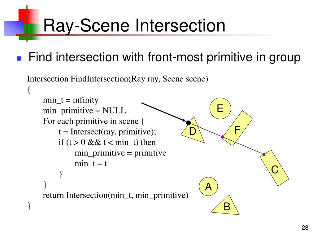
The algorithm, which you've already implemented within the hittable_list::hit method, follows these steps:

1. Initialize a variable, closest_so_far, to the maximum renderable distance (ray_tmax).
2. Iterate through each object in the list.
3. For each object, call its hit method, but with an important constraint: the new maximum distance is closest_so_far.
4. If a hit is found that is closer than closest_so_far, update closest_so_far to this new, smaller distance and record the details of this hit.
5. After checking all objects, the recorded hit details will be for the closest object.

This pattern is fundamental to ray tracing. To reinforce the concept, let's look at how another resource describes this exact logic.

The trace function in the article does exactly what our hittable_list::hit method does. Now, let's integrate our class into the main program.

Updating the Main Program to Render a Scene

Our primary guide for implementation, Ray Tracing in One Weekend, has a chapter dedicated to this integration. We will now follow its steps to bring our scene to life.

Let's summarize the key steps to modify in your main.cc file:

1. Create the World and Add Objects

In your main() function, before your main render loop, instantiate hittable_list and add a couple of spheres. This uses the std::vector and std::shared_ptr concepts we covered earlier.

// In main()
hittable_list world;

world.add(make_shared<sphere>(point3(0, 0, -1), 0.5));
world.add(make_shared<sphere>(point3(0, -100.5, -1), 100));

Here, we've created two spheres. The second one is very large and positioned below the camera, which will serve as a simple ground plane.

2. Modify ray_color() Signature

Your ray_color() function currently probably takes a reference to a single hittable object. We need to generalize it to take the entire world.

Change its signature from something like color ray_color(const ray& r, const sphere& s) to:

color ray_color(const ray& r, const hittable& world)

3. Update the ray_color() Logic

Inside ray_color(), replace the call to the specific object's hit method with a call to the world's hit method.

// Inside ray_color()
hit_record rec;

// The original 't_max' is infinity, meaning we're interested in any hit, no matter how far.
// We check for hits from t=0.0 to infinity.
if (world.hit(r, 0.0, infinity, rec)) {
    // If we hit something, color based on its normal.
    return 0.5 * (rec.normal + color(1, 1, 1));
}

// If we hit nothing, return the background color.
vec3 unit_direction = unit_vector(r.direction());
auto a = 0.5 * (unit_direction.y() + 1.0);
return (1.0 - a) * color(1.0, 1.0, 1.0) + a * color(0.5, 0.7, 1.0);

(Note: You'll need to include the header for your hittable_list in main.cc)

4. Update the Call in the Main Loop

Finally, in your main rendering loop where you call ray_color for each pixel, make sure you pass the world object.

// Inside the nested for loops in main()
// ...
color pixel_color = ray_color(r, world);
write_color(std::cout, pixel_color);

After making these changes, compile and run your program. You should see your first multi-object render: a small sphere appearing to float above a much larger one that acts as the ground.

Visualizing the Process

To see this process in action from a different perspective, let's watch a segment from The Cherno's series. His implementation details differ slightly (he puts the loop in the main trace function rather than a class method), but the core logic of iterating and finding the minimum hit_distance is identical.

Conclusion

Congratulations! You have successfully configured your renderer to trace rays against an entire scene of objects. This is a monumental step that transforms your project from a simple geometric calculator into a scalable rendering system.

Key Takeaways:

• By creating a hittable_list and populating it in main, you've defined your first "scene" or "world."
• The ray_color function is now generalized; it operates on the abstract hittable interface, not a concrete object type. It doesn't care if the "world" is one sphere or a million triangles in a complex model.
• The core algorithm for finding the visible surface is to iterate through all objects and find the intersection with the smallest positive t value. This logic is now encapsulated and working within your hittable_list::hit method.

Your work today connects directly to how production renderers operate, albeit at a much simpler scale. Renderers like Arnold and Karma manage vast scenes containing millions or billions of primitives. Simply looping through every object, as we do now, would be impossibly slow. In a future module, we will explore acceleration structures (like the BVH you may have heard of) which are essential for making such scenes render in a reasonable amount of time.

Next Steps

Take a close look at the image you just rendered. Do you see the sharp, jagged edges along the silhouette of the sphere? This artifact is called aliasing. In our next lesson, we will investigate its cause and implement a fundamental technique to combat it: multi-sample anti-aliasing.