Sphere Intersection Normal Vector Calculation

From Intersection Distance t to a 3D Hit Point

First things first. We have the distance t, but we need the actual 3D coordinates of the intersection point. Fortunately, this is a direct application of the ray's parametric equation, which you know well:

$\mathbf{P}(t)=\mathbf{O}+t\mathbf{D}$

Where $\mathbf{P}$ is a point on the ray, $\mathbf{O}$ is the ray's origin, and $\mathbf{D}$ is its direction. Since our hit_sphere function now returns the correct value of t for the closest intersection, we can find the world-space hit point, ${\mathbf{P}}_{\text{hit}}$, by simply plugging t into the equation.

// Assuming 'r' is our ray and 't' is the value from hit_sphere
point3 P_hit = r.at(t); // or r.origin() + t * r.direction();

This simple step is powerful; it translates our 1D distance t into a full 3D coordinate. This point is where all our subsequent shading calculations will happen.

What is a Surface Normal?

Before we calculate it, let's clarify what a surface normal is. A surface normal (or just "normal") is a vector that is perpendicular to the surface at a specific point. It essentially tells you which direction the surface is "facing" at that location.

Think about standing on a smooth hill. The direction pointing straight up from the ground beneath your feet is the surface normal at your position. As you walk around, the normal's direction changes, always pointing away from the surface. In graphics, this vector is the key to figuring out how light should reflect off a surface.

To get a solid intuition for this concept and why it's so critical for lighting, please watch the following segment.

Calculating the Normal for a Sphere

For some complex shapes, calculating the normal can be mathematically intensive. For a sphere, however, it's beautifully simple. The vector from the center of a sphere to any point on its surface is, by definition, perpendicular to the surface at that point.

This gives us a straightforward formula:

$\mathbf{N}=\frac{{\mathbf{P}}_{\text{hit}}-{\mathbf{C}}_{\text{sphere}}}{||{\mathbf{P}}_{\text{hit}}-{\mathbf{C}}_{\text{sphere}}||}$

In words: subtract the sphere's center from the intersection point, and then normalize the resulting vector. Normalizing it (making its length 1) is a critical convention. It turns the vector into a pure direction, which simplifies lighting equations later on. This policy is explained well in Ray Tracing in One Weekend.

The resource below from Scratchapixel provides the same formula and a concise code snippet, reinforcing the concept.

Putting It Into Practice: Visualizing Normals

We now have the theory to calculate the normal. But how do we check if our code is correct? We can't just print out millions of vectors. A common and powerful technique in graphics programming—one you've likely encountered in your VFX work with things like "normal passes"—is to visualize data as color.

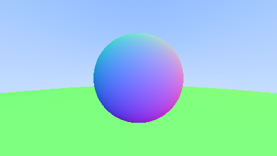
We can map the X, Y, and Z components of our normal vectors directly to the R, G, and B channels of our output image. There's one small catch: normal components are in the range [-1, 1], while color components need to be in [0, 1]. We can remap the range with a simple linear transformation:

$\text{pixel\_color}=0.5\times (\mathbf{N}+\text{vec3}(1,1,1))$

For example, a normal component of -1 becomes 0.5 * (-1 + 1) = 0, and a component of 1 becomes 0.5 * (1 + 1) = 1. This neatly scales our normal into a visible color range.

The following resources show exactly how to implement this, bringing our concepts together into working code.

The C++ code in Ray Tracing in One Weekend provides a perfect template for updating our ray_color function.

Your Updated ray_color Function

By combining these ideas, your ray_color function should now look something like this:

color ray_color(const ray& r) {
    // In the last lesson, we created this function. Now we'll use its return value.
    auto t = hit_sphere(point3(0, 0, -1), 0.5, r);

    // If the ray hits the sphere...
    if (t > 0.0) {
        // Calculate the hit point using the 't' value.
        point3 hit_point = r.at(t);
        // Calculate the normal at the hit point.
        vec3 normal = unit_vector(hit_point - point3(0, 0, -1));
        // Map the normal's [-1, 1] components to [0, 1] color range and return it.
        return 0.5 * color(normal.x() + 1, normal.y() + 1, normal.z() + 1);
    }

    // If the ray misses, return the background color.
    vec3 unit_direction = unit_vector(r.direction());
    auto a = 0.5 * (unit_direction.y() + 1.0);
    return (1.0 - a) * color(1.0, 1.0, 1.0) + a * color(0.5, 0.7, 1.0);
}

When you run this, you should see a colorful sphere, where red corresponds to the X-axis, green to the Y-axis, and blue to the Z-axis.

Conclusion

Excellent work! You have now connected all the dots from ray-casting to surface analysis. This is a major milestone. You're no longer just detecting objects; you're extracting essential geometric information from them.

Key Takeaways:

• The 3D intersection point is found by plugging the t value from your intersection test into the ray equation: $\mathbf{P}=\mathbf{O}+t\mathbf{D}$.
• A surface normal is a unit vector perpendicular to a surface, indicating the direction it faces.
• For a sphere, the normal is calculated by subtracting the sphere's center from the hit point and normalizing the result: $\mathbf{N}=\text{normalize}({\mathbf{P}}_{\text{hit}}-{\mathbf{C}}_{\text{sphere}})$.
• Visualizing normals by mapping their [-1, 1] components to [0, 1] RGB colors is a powerful debugging technique.

Next Steps

The next official learning outcome is to "visualize surface normals as colors," which we've already covered as a necessary verification step. In our next lesson, we will formalize this, ensure our code is robust, and then move right on to a topic you've been waiting for: Module 4: Positionable Camera and Scene View. We'll use our knowledge of vectors to build a complete camera system that can be positioned anywhere in the scene, looking at any point, preparing you to explore more complex worlds.