Debugging Normals with Color

Why Visualize Normals? The Power of Visual Debugging

When writing a ray tracer, you're dealing with millions of pixels, each with its own ray, potential intersections, and calculated data. Trying to verify this by printing numbers to a console is impractical. By mapping data like a normal vector to an RGB color, you gain immediate, intuitive insight into your program's behavior across the entire image.

• A smooth, colorful gradient across a curved surface tells you the normals are being calculated correctly.
• Sudden, sharp changes in color or bizarre patterns can instantly flag bugs in your intersection math or normal calculation.

This practice of outputting data as colors is a cornerstone of graphics debugging.

The Technique: Mapping a Vector to a Color

As we discussed, the core idea is to map the three components of a normal vector $(N_x,N_y,N_z)$ to the three channels of an RGB color $(R,G,B)$.

A normal is a unit vector, so its components lie in the range $[-1,1]$. However, color channels are typically represented in the range $[0,1]$. We need a simple transformation to map one range to the other.

The formula for this is:
$\text{color}=0.5\times (\text{normal}+\mathbf{v})$
where $\mathbf{v}$ is a vector of $(1,1,1)$. This scales the $[-1,1]$ range down to $[-0.5,0.5]$ and then shifts it up by 0.5, resulting in the desired $[0,1]$ range.

To see this in action and reinforce your understanding, the following video explains and implements this exact technique.

Refactoring for Cleaner Intersections

In our previous code, the hit_sphere function returned a single double representing the intersection distance t. This was simple, but it forced our main ray_color function to recalculate the hit point and the normal. A much cleaner, more scalable approach is to have the intersection function return all the relevant data in one package.

This is where a hit_record struct comes in. It's a simple container for all the information about a ray-object intersection:

• point3 p: The 3D coordinates of the intersection point.
• vec3 normal: The surface normal at the intersection point.
• double t: The ray parameter t of the intersection.

Let's see how the Ray Tracing in One Weekend series introduces this concept. This is a crucial step towards building an abstraction for any object that can be hit by a ray, which we'll tackle in a future module.

With this hit_record struct, we can refactor our hit_sphere function. Instead of returning a double, it will now return a bool (indicating if a hit occurred) and populate a hit_record passed by reference.

Here is what the signature and logic would look like:

// Before
double hit_sphere(const point3& center, double radius, const ray& r);

// After
bool hit_sphere(const point3& center, double radius, const ray& r, hit_record& rec);

Inside the new hit_sphere function, if you find a valid intersection at distance t, you would then populate the rec object:

// ... inside hit_sphere, after finding a valid root 't' ...
rec.t = root;
rec.p = r.at(rec.t);
vec3 outward_normal = (rec.p - center) / radius;
rec.normal = outward_normal; // We'll refine this part in a later lesson
return true;

Putting It All Together: The Final Image

Now, we can update our ray_color function to use this new, cleaner structure. It no longer needs to calculate the normal itself; it just receives it from the hit_record.

The updated code flow is much clearer:

1. Check for an intersection using the new hit_sphere function.
2. If there's a hit, the hit_record is now filled with data.
3. Use rec.normal and our remapping formula to return the final color.

The book Ray Tracing in One Weekend provides the definitive implementation of this.

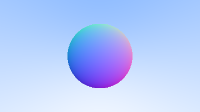
After implementing these changes, your rendered image should look like this, confirming that your normal calculations are correct for every point on the sphere.

Conclusion

Congratulations! You have now mastered a fundamental debugging technique in computer graphics and have made your intersection code more robust and scalable. This is a crucial checkpoint before we start building more complex scenes.

Key Takeaways:

• Visualizing data, especially vectors like normals, by mapping them to colors is an essential and powerful method for debugging graphics code.
• The mapping from a normal's $[-1,1]$ component range to a color's $[0,1]$ range is achieved with the simple formula: color = 0.5 * (normal + vec3(1, 1, 1)).
• Refactoring your intersection functions to use a hit_record struct to return all intersection data is a cleaner, more scalable design that you will build upon throughout this course.

Next Steps

With our sphere intersection and normal visualization code on solid footing, we are now ready to tackle the topic you expressed interest in early on: building a flexible camera system. In the next lesson, we will begin Module 4: Positionable Camera and Scene View. You will learn how to:

• Define a camera's position and orientation in 3D space using lookfrom, lookat, and view-up vectors.
• Implement an adjustable field of view to control the camera's zoom.

This will empower you to move around your scene and view your creations from any angle, a significant step towards creating compelling 3D images.