Sample Size Determination Using Power Analysis

The Four Pillars of Power Analysis

An a priori power analysis, which is performed before data collection to determine the necessary sample size, relies on the relationship between four key parameters. When you specify any three, the fourth is determined. For our purpose, we will set three to solve for the fourth: sample size.

1. Significance Level ($\alpha$): This is the probability of a Type I error—rejecting the null hypothesis when it is true. In our context, it's the risk of concluding that there is a difference in appeal between bra styles when, in reality, there isn't one. We will adhere to the standard convention of $\alpha =0.05$.

2. Statistical Power ($1-\beta$): This is the probability of correctly rejecting the null hypothesis when it is false. It's the likelihood that our experiment will detect a true difference in appeal scores if one exists. A common target for power is 0.80 (or 80%), which means we accept a 20% chance of a Type II error ($\beta$).

3. Effect Size (f): This quantifies the magnitude of the difference between groups you expect to find. It is a standardized measure, meaning it's independent of the scale of your dependent variable. For ANOVA, this is typically Cohen's f. This is the most critical and often most subjective input.

4. Sample Size (N): This is the total number of observations (ratings) we need to collect across all groups. This is what we aim to calculate.

The following resource provides a solid conceptual review of these pillars.

Defining Effect Size: What's a "Meaningful" Difference?

The heart of a power analysis lies in defining the effect size. How large of a difference between your lingerie styles do you actually care about detecting? A very subtle difference might require hundreds of ratings to prove statistically, while a dramatic difference can be detected with a much smaller sample.

There are three primary ways to determine the effect size for your experiment:

1. From a Pilot Study: The most robust method is to use data from a small preliminary study. For instance, you could collect 5-10 appeal ratings for each bra style. From this data, you can calculate the mean score for each style and the common standard deviation, which can then be used to calculate Cohen's f.

2. Based on Practical Significance: You, as the designer, can define the smallest difference that you would consider meaningful. For example, on a 10-point appeal scale, you might decide that a difference of less than 1 point between styles is not practically important. You can combine this target difference with an estimate of the score variability (standard deviation) to calculate the effect size.

3. Using Conventions: When no prior data is available, you can fall back on Cohen's established conventions for effect size f:

   • Small effect (f = 0.10): A subtle but detectable difference.
   • Medium effect (f = 0.25): A difference large enough to be apparent to a careful observer.
   • Large effect (f = 0.40): A substantial and readily noticeable difference.

The following resource walks through how these different effect sizes dramatically impact the required sample size.

Performing the Analysis with G*Power

G*Power is a free and widely used tool for conducting power analyses. We will use it to perform an a priori analysis for our one-way ANOVA design. Let's return to our experiment comparing three bra styles: push-up, balconette, and plunge.

The process in G*Power is straightforward:

• Test family: Select F tests.
• Statistical test: Select ANOVA: Fixed effects, omnibus, one-way.
• Type of power analysis: Select A priori: Compute required sample size.

This sets up the calculator, which requires the four pillar inputs. Let's run two scenarios.

Scenario 1: Detecting a "Medium" Effect

Assume you're looking for a moderately apparent difference in appeal. We will use the conventional medium effect size.

• Input Parameters:
  • Effect size f: 0.25 (Cohen's medium)
  • α err prob: 0.05
  • Power (1-β err prob): 0.80
  • Number of groups: 3

After you enter these values and click "Calculate," G*Power provides the required sample size. The article we reviewed earlier provides a clear walkthrough of this exact process.

Scenario 2: Detecting a "Small" Effect

What if you suspect the differences are more subtle? Let's see what happens if we aim to detect a small effect.

• Input Parameters:
  • Effect size f: 0.10 (Cohen's small)
  • All other parameters remain the same ($\alpha =0.05$, Power=0.80, Groups=3).

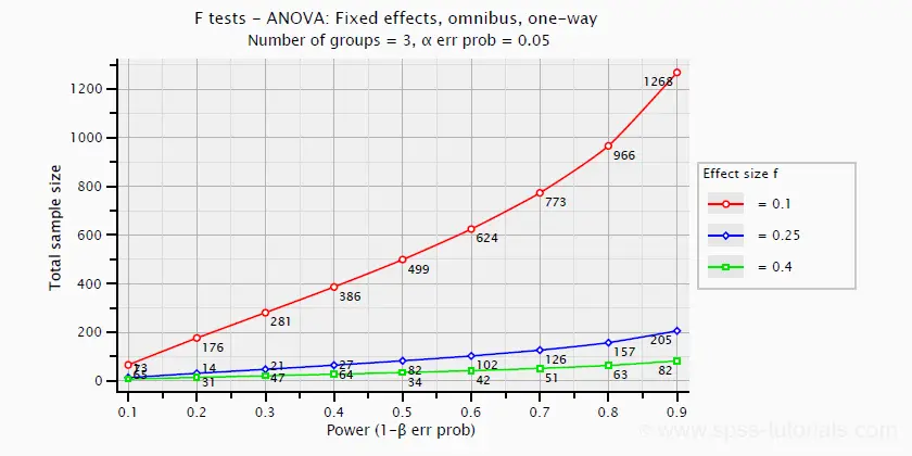
Recalculating in G*Power with this new effect size yields a total sample size of 969 ($323$ per style). This tenfold increase in required sample size for a smaller effect underscores why defining your effect size is the most consequential step in power analysis.

The graph below visualizes this relationship. For a given level of power (x-axis), the required sample size (y-axis) explodes as the effect size you want to detect gets smaller.

Practice Exercise

Now it's your turn. You are planning the experiment from the last lesson, comparing four lingerie bottom styles: thong, brazilian, boyshort, and high-waist. The dependent variable is a 'versatility score' (1-20 scale).

From a small pilot study, you estimate the common standard deviation ($\sigma$) of the scores to be 4 points. You decide that a difference is only practically meaningful if the mean scores of the styles are spread out. Specifically, you want to be able to detect an effect if the mean scores are 12, 14, 16, and 18.

1. Use G*Power to calculate the effect size f.
   • Hint: In the main window, click the "Determine" button. Select "Effect size from means" and input your number of groups, the common SD, and the group means.
2. With that effect size, determine the total sample size needed to achieve 90% power ($1-\beta =0.90$) with $\alpha =0.05$.
3. In practice, some data may be lost or unusable. Adjust the calculated sample size to account for an anticipated 10% drop-out rate.
   • Hint: $N_{\text{final}}=N/(1-\text{drop-out rate})$

Jot down your answers for the calculated effect size, the initial total sample size, and the final adjusted sample size.

Conclusion

You have now learned how to bridge the gap between experimental design and practical execution. By performing a power analysis, you can make an informed decision about the sample size needed for your lingerie comparison experiments, ensuring your study is both efficient and has a high probability of detecting a true effect.

Key Takeaways:

• Power analysis is a critical step to determine the required sample size for an experiment, balancing the risk of Type I ($\alpha$) and Type II ($\beta$) errors.
• The required sample size is highly sensitive to the effect size (f), which quantifies the magnitude of the difference you aim to detect.
• Estimating effect size can be done using pilot data, practical significance, or established conventions.
• Tools like G*Power automate the calculation, allowing you to focus on the critical task of defining the experimental parameters.

In our previous lesson, we designed the experiment. Today, we determined how many observations to collect. In our next lesson, we will analyze the data. After running the ANOVA and finding a significant result, we will need to know which specific styles differ from each other. We will accomplish this by learning how to conduct and interpret post-hoc tests, such as Tukey's HSD.