Welcome back. In our previous lessons, we designed a one-way ANOVA experiment to compare different lingerie styles and then performed a power analysis to determine the necessary sample size for that experiment. We now move to the next logical step: analyzing the data you've collected.
Imagine you've completed your fitting room trials, gathered the appeal scores for your bra styles, and now have a dataset ready for analysis. The central question remains: is there a statistically significant difference in appeal among the styles? This lesson will teach you how to answer that question by interpreting the primary output of an ANOVA: the F-statistic and its corresponding p-value. This is the crucial "omnibus" test that tells you whether your experiment detected a genuine effect or just random noise.
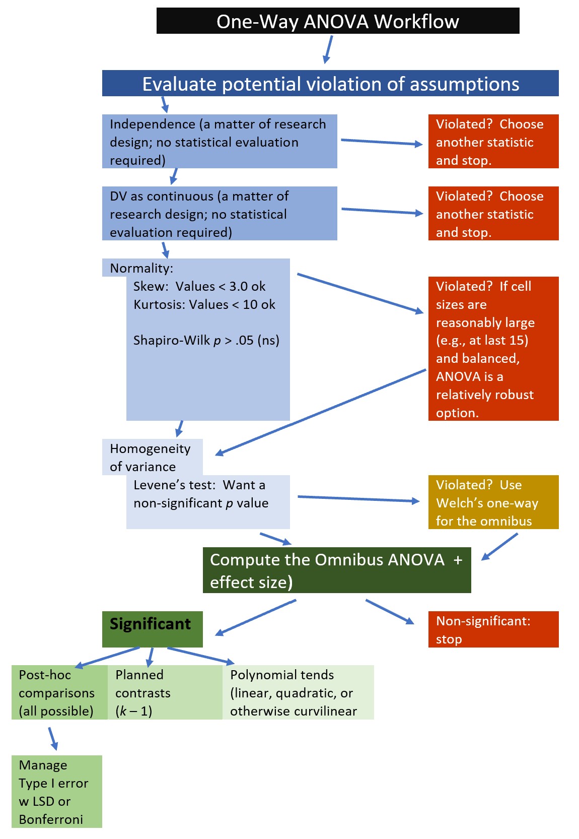
The ANOVA Workflow: From Data to Decision
The entire process of conducting a one-way ANOVA can be visualized as a decision-making workflow. We have already covered the initial assumption checks in our discussion of experimental design. Today, we focus on the core computational step and the subsequent decision point.
The Logic of ANOVA: Signal vs. Noise
Given your background in experimental design, you'll recall that ANOVA's power lies in its method of partitioning variance. It essentially asks whether the variation between the groups you are comparing is larger than the variation within those groups.
Let's frame this in our lingerie context, comparing three bra styles: push-up, balconette, and plunge.
-
Between-Group Variation (The "Signal"): This measures how much the mean appeal scores of the three bra styles differ from one another. If the push-up style is consistently rated higher than the balconette, this contributes to the between-group variation. This is the potential effect of your design choice—the "signal" you are looking for.
-
Within-Group Variation (The "Noise"): This measures the natural variability of scores within a single style. Not everyone will give the push-up bra the same score; some will love it, some may be indifferent. This random, unexplained variability is considered statistical "noise."
The F-statistic is the elegant ratio of these two sources of variation:
If the different bra styles have no real effect on appeal, the "signal" should be about the same size as the "noise," and the F-statistic will be close to 1.0. However, if one or more styles are genuinely more appealing, the signal will be stronger than the noise, yielding an F-statistic significantly greater than 1.0.
The following resource provides an excellent, concise explanation of this logic and the components that go into the calculation.
Interpreting results: One-way ANOVA
This guide from GraphPad clearly explains the core principles of ANOVA.
Please read the sections How ANOVA works and Mean squares. Focus on how the total variation (Sum of Squares Total) is partitioned into variation between the styles and variation within the styles, and how these are converted to Mean Squares (variances).
Deconstructing the ANOVA Table
The results of an analysis of variance are traditionally presented in an ANOVA table. This table neatly organizes the components of variation we just discussed. Let's imagine we ran our experiment comparing the push-up, balconette, and plunge styles, with 10 ratings collected for each style (a total of N=30 ratings). The output from our statistical software would look something like this:
| Source | SS | df | MS | F | p-value |
|---|---|---|---|---|---|
| Between Groups | 50.0 | 2 | 25.0 | 6.25 | 0.005 |
| Within Groups | 108.0 | 27 | 4.0 | ||
| Total | 158.0 | 29 |
Let's break down each column:
- Source: Identifies the component of variation. "Between Groups" is our signal (the effect of bra style), and "Within Groups" is our noise (random error).
- SS (Sum of Squares): Represents the total variation attributable to each source. You can see that SS(Between) + SS(Within) = SS(Total).
- df (Degrees of Freedom): The number of independent pieces of information used to calculate the SS.
df(Between)= , where is the number of groups. Here, .df(Within)= , where is the total number of observations. Here, .
- MS (Mean Square): This is the average variation, or variance, for each source. It's calculated as
MS = SS / df. This is the value we use for the F-ratio.MS(Between)is our signal variance, andMS(Within)is our noise variance. - F (F-statistic): The critical value we've been building towards. It's calculated as
F = MS(Between) / MS(Within). In our table, . - p-value: The probability of observing an F-statistic of 6.25 or higher if there were actually no difference between the styles.
Making the Decision: Interpreting F and p
Now we arrive at the decision point. To interpret these results, we must first state our hypotheses.
- Null Hypothesis (H₀): There is no difference in the mean appeal scores among the three bra styles in the population. ()
- Alternative Hypothesis (H₁): At least one of the bra styles has a different mean appeal score from the others.
We use the p-value to decide whether to reject H₀. Using a standard significance level () of 0.05:
- Our calculated F-statistic is 6.25. This is substantially larger than 1.0, suggesting the signal is stronger than the noise.
- The associated p-value is 0.005.
Conclusion: The probability of observing such a large difference between our bra styles purely by chance is very low (0.5%). Since , we reject the null hypothesis. We have statistically significant evidence to conclude that the choice of bra style has an effect on its appeal score.
This significant result is our green light to proceed. It confirms that our experiment was successful in detecting a difference. However, it's crucial to remember what this result doesn't tell us. We know that a difference exists, but we don't know where. Is the plunge bra significantly better than the balconette? Is there no difference between the push-up and plunge? The omnibus ANOVA test cannot answer these questions.
The following reading reinforces how to draw conclusions from the F-ratio and p-value.
Interpreting results: One-way ANOVA
This part of the guide focuses directly on the interpretation of the key results.
Please read the sections The null hypothesis, The F statistic, and P value. This will solidify your understanding of how these three components work together to yield a conclusion.
Practice Exercise
Now it's your turn to interpret the results. Let's say you've completed the experiment from our last lesson's exercise, comparing four lingerie bottom styles: thong, brazilian, boyshort, and high-waist. You collected appeal scores from a total of 80 participants (20 per style). Your analysis produced the following ANOVA table, with some values missing.
| Source | SS | df | MS | F | p-value |
|---|---|---|---|---|---|
| Between Groups | 180.0 | ? | ? | ? | 0.02 |
| Within Groups | 1520.0 | ? | ? | ||
| Total | 1700.0 | 79 |
Your Task:
- Calculate the missing values in the table:
df(Between),df(Within),MS(Between),MS(Within), and theF-statistic. - State the null hypothesis (H₀) for this specific experiment comparing the four bottom styles.
- Using a significance level of , what is your conclusion? Write a one-paragraph summary explaining what this result means for your lingerie design project. Do you stop here, or do you proceed with more analysis?
Take your time to fill in the table and formulate your conclusion.
Conclusion
In this lesson, you've learned to interpret the core output of a one-way ANOVA. You can now take the raw data from your experiments, analyze it, and make a statistically-backed decision about whether a significant difference exists among your designs.
Key Takeaways:
- The ANOVA table systematically breaks down the total variation in your data into "signal" (Between-Group variation) and "noise" (Within-Group variation).
- The F-statistic is a ratio of the signal to the noise. A value significantly greater than 1 suggests a real effect is present.
- The p-value gives the probability of observing your data if the null hypothesis (of no difference) were true. A p-value less than your chosen alpha level () allows you to reject the null hypothesis.
- A significant ANOVA result is an "omnibus" finding. It tells you that at least one group is different from the others, but not which specific groups differ.
This brings us to the next critical question. Now that we have evidence that not all bottom styles are rated equally, how do we find out exactly which ones are the winners and losers? In our next lesson, we will cover post-hoc tests, such as Tukey's HSD, which allow us to perform pairwise comparisons to pinpoint exactly where the significant differences lie.