Welcome back. In our last lesson, we began our exploration of Principal Component Analysis, focusing on how PCA transforms a complex set of features into a smaller number of principal components. We saw how to use rotated component loadings to interpret and assign meaningful, design-relevant names to these new dimensions, such as "Structural Support" or "Delicate Ornamentation."
This lesson builds directly on that foundation. Knowing what the components represent is half the battle; the other half is deciding how many of them are actually worth keeping. Retaining too few components risks throwing away valuable information about style variations, while keeping too many defeats the purpose of dimensionality reduction by including noise. Today, we will focus on the tools and criteria used to make this critical decision. You will learn to interpret scree plots and apply established rules to determine the optimal number of components to retain. We will also deepen your understanding of component loadings by visualizing them.
Deciding How Many Components to Retain
After running a PCA on a dataset with p original features, you get back p principal components. The key is that they are not created equal. They are ordered by the amount of variance they explain, from most to least. Our task is to find the point of diminishing returns, where the components stop representing meaningful signals and start representing noise.
The primary tool for this is the scree plot. This is a simple but powerful graph that plots the eigenvalue (or the percentage of variance explained) for each principal component in descending order.
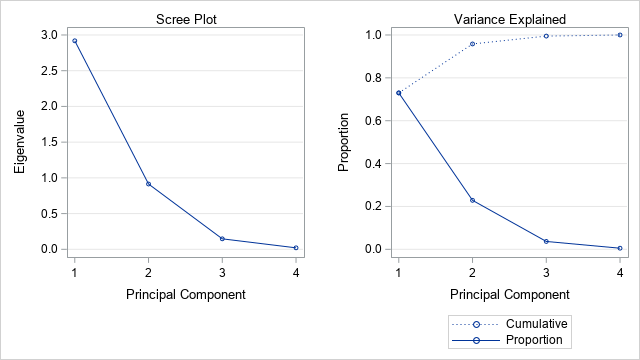
By examining the shape of this plot, we can decide where to "cut off" the number of components. There are three common heuristics for doing this, which you'll find complement each other well.
1. The Elbow Rule
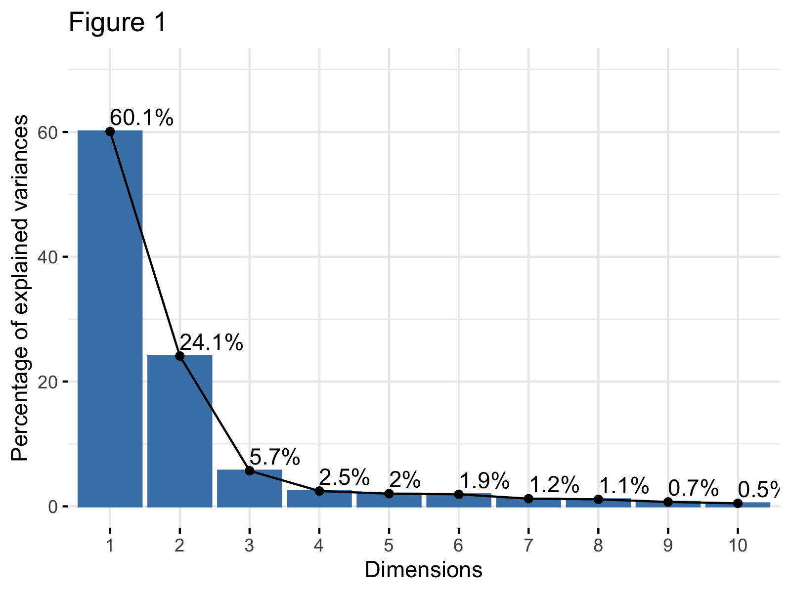
This is a visual method. You look for a bend, or "elbow," in the scree plot. The components to the left of the elbow are the ones that explain the most variance. The components to the right, where the line flattens out, are considered "scree"—the geological debris at the bottom of a cliff—and are generally discarded.
2. The Kaiser Criterion
Since you are familiar with the underlying mechanics of PCA, you know that eigenvalues represent the amount of variance captured by each component. When PCA is performed on standardized data (which is standard practice), the average eigenvalue is 1. The Kaiser criterion suggests a simple rule: keep only the components with an eigenvalue greater than 1. The intuition is that a principal component should explain at least as much variance as a single one of the original variables. In the "Scree Plot" image above, this rule would lead us to keep the first two components, as their eigenvalues are approximately 2.9 and 0.9, but Component 2 is close enough that further inspection is warranted.
3. Cumulative Proportion of Variance
This is a more pragmatic approach. You decide on a satisfactory level of variance you wish to explain—a common threshold is between 80% and 90%—and you keep the smallest number of components required to meet that threshold. Looking at the "Variance Explained" plot above, you can see that PC1 explains about 73% of the variance. PC1 and PC2 together explain about 96% (the second point on the "Cumulative" line). If your goal was to explain at least 80% of the variance, you would need to keep two components.
This DataCamp tutorial provides a very clear summary and practical R code examples for these concepts.
Principal Component Analysis (PCA) in R Tutorial
This tutorial provides a concise walkthrough of PCA, including how to generate and interpret the key outputs for deciding how many components to retain.
Please read the following sections: First, review the section on the Scree Plot. It shows how to generate one and interpret it. Next, read the section "How to choose the number of components," which explicitly summarizes the Elbow rule and the Variance threshold. Finally, the FAQ at the end also provides a good reinforcement under the question "How do I choose the number of principal components?", which also introduces the Kaiser criterion.
Visualizing and Interpreting Loadings with a Biplot
In the previous lesson, we interpreted loadings from a table. While effective, it can be more intuitive to visualize them. A biplot is a graph that overlays the component scores of the observations with the component loadings of the variables. This allows you to see how individual data points (e.g., specific lingerie pieces) relate to the underlying style dimensions.
The loadings are represented by vectors (arrows) originating from the center (0,0). Here’s how to interpret them:
- Direction: The angle between vectors indicates the correlation between the original variables. Vectors pointing in similar directions represent positively correlated variables. Vectors pointing in opposite directions represent negatively correlated variables. Orthogonal vectors represent uncorrelated variables.
- Length: The length of a vector indicates how well that variable is represented by the two plotted components. Longer vectors mean the variable is well-explained by the two dimensions; shorter vectors suggest that other components (not plotted) are needed to explain their variance.
Let's look at how to use a biplot in practice.
Principal Component Analysis (PCA) in R Tutorial
This part of the tutorial explains how to generate and interpret a biplot. The concept of Cos2 (squared cosine) is also introduced as a measure of representation quality.
Please read the sections titled "Biplot of the attributes" and "Contribution of each variable." Focus on how the biplot visually represents the information we previously read from the loading matrix and what Cos2 tells us.
A Practical Example: Anthropometric Data
The paper on clothing size prediction offers a clear, published example of these steps in action. The researchers used PCA on a large set of body measurements to identify key body shape factors.
Evaluating machine learning models for clothing size prediction ...
This paper applies the exact methods we are discussing to a related field. It provides a good model for how you would report and justify your own PCA findings.
Please read the three short subsections under "SVM model for size prediction via multiple body measurements": "Variance explained": Note their result—three components explained 86.4% of the variance. "Scree plot": See how they use the scree plot and its "sharp elbow" to justify their decision to retain three components. "Rotated component matrix": This is exactly what we did in the last lesson. They interpret their three retained components as representing "horizontal measurements," "height," and "body width," respectively.
This example mirrors the process you would follow: run PCA, use the scree plot and variance explained to select the number of components, and then interpret the loadings of those components to define your core lingerie style dimensions.
Numerical Exercise: Defining Bikini Style Dimensions
Imagine you have analyzed a collection of 50 bikini styles based on six design features. You've run a PCA and obtained the following results for the eigenvalues and the rotated component loading matrix.
PCA Results:
| Component | Eigenvalue | % of Variance | Cumulative % |
|---|---|---|---|
| 1 | 2.82 | 47.0% | 47.0% |
| 2 | 1.98 | 33.0% | 80.0% |
| 3 | 0.54 | 9.0% | 89.0% |
| 4 | 0.36 | 6.0% | 95.0% |
| 5 | 0.24 | 4.0% | 99.0% |
| 6 | 0.06 | 1.0% | 100.0% |
Rotated Component Loadings:
| Feature | Component 1 | Component 2 |
|---|---|---|
Triangle_Coverage |
-0.91 | 0.08 |
Strap_Thickness |
-0.85 | 0.15 |
Underboob_Cutout |
0.88 | -0.11 |
Fabric_Shimmer |
0.05 | 0.94 |
Color_Vibrancy |
0.12 | 0.90 |
Hardware_Accents |
-0.09 | 0.82 |
Your task is to analyze these results.
- How many components should you retain? Justify your decision using two different criteria from the lesson (e.g., Kaiser criterion and Cumulative Variance).
- Interpret the retained components. Based on the loading matrix, provide a descriptive name for Component 1 and Component 2 that captures their essence in bikini design terms.
- Describe a bikini style that would have a high positive score on Component 1 and a low score on Component 2.
- Describe a bikini style that would have a high positive score on Component 2 and a low score on Component 1.
Take your time to analyze the tables and formulate your answers.
Click for a detailed solution.
Here is a step-by-step analysis:
-
Number of Components to Retain:
- Kaiser Criterion: This rule suggests keeping components with eigenvalues greater than 1. Here, Component 1 (eigenvalue = 2.82) and Component 2 (eigenvalue = 1.98) meet this criterion. Component 3 has an eigenvalue of 0.54, which is well below the cutoff. This method suggests retaining 2 components.
- Cumulative Variance Explained: A common goal is to explain at least 80% of the variance. The table shows that the first two components together explain exactly 80.0% of the total variance. To exceed this, we'd need more, but hitting it exactly is often considered sufficient. Retaining a third component only adds 9% more information at the cost of increased complexity. Therefore, retaining 2 components is a very reasonable choice.
- (Note: A scree plot of these eigenvalues would also show a clear "elbow" after the second component, further supporting this decision).
-
Interpret and Name the Components:
- Component 1: This component has strong positive loadings for
Underboob_Cutout(0.88) and strong negative loadings forTriangle_Coverage(-0.91) andStrap_Thickness(-0.85). This dimension clearly contrasts revealing styles (cutouts, less coverage, thin straps) with more conservative, fuller-coverage styles. A suitable name would be "Coverage vs. Reveal" or "Modesty vs. Audacity". A high score indicates a more revealing style. - Component 2: This component is defined by high positive loadings for
Fabric_Shimmer(0.94),Color_Vibrancy(0.90), andHardware_Accents(0.82). This dimension is all about visual impact, decoration, and eye-catching details. A good name would be "Visual Pop" or "Glam Factor". A high score indicates a more visually striking style.
- Component 1: This component has strong positive loadings for
-
High PC1, Low PC2:
A bikini with a high positive score on Component 1 would be very revealing (e.g., significant underboob cutout, minimal triangle coverage, very thin straps). A low score on Component 2 means it would be visually subtle (e.g., a matte fabric, a neutral or muted color, no metallic hardware). This describes a minimalist, high-cut, "barely there" style in a plain fabric. -
High PC2, Low PC1:
A bikini with a high positive score on Component 2 would be very flashy (e.g., made of a high-shimmer fabric in a neon color, with decorative gold rings or clasps). A low score on Component 1 (which means a negative value, since PC scores are centered at 0) would mean it has high coverage and thicker straps. This describes a supportive, full-coverage bikini top in a vibrant, glittery fabric with prominent hardware.
Conclusion
In this lesson, you have learned the critical process of determining the appropriate number of principal components to retain in your analysis. This decision is a crucial balance between model simplicity and information richness. You are now equipped with a set of practical tools and criteria to make a well-justified choice.
Key Takeaways:
- Scree plots are the primary visual tool for assessing the importance of each principal component.
- You can decide how many components to keep using the Elbow Rule (where the plot flattens), the Kaiser Criterion (eigenvalue > 1), or by targeting a specific Cumulative Percentage of Variance Explained (e.g., 80-90%).
- A biplot offers an intuitive way to visualize component loadings, revealing the relationships between original features and their alignment with the principal components.
So far in this module, we have taken a dataset with many features, reduced its dimensionality by identifying the core "style dimensions" with PCA, and learned how to interpret those dimensions. In our next lesson, we will put these new dimensions to work. We will use them as the input for hierarchical clustering, an algorithm that can automatically group your lingerie pieces into distinct, data-driven style families.