Welcome to the first lesson of our new module on segmenting lingerie styles. In the previous module, we focused on understanding the relationships between pairs of variables, using tools like Pearson and Spearman correlation to measure the association between a design feature and its appeal. Now, we will move from analyzing variables two at a time to exploring the overall structure of a dataset with many features at once.
Imagine you have a collection of lingerie pieces, each described by a dozen attributes: cup coverage, strap width, fabric sheerness, lace percentage, color saturation, and so on. Many of these features are likely correlated. For instance, high lace percentage might often go with high fabric sheerness. How can you see past this complexity to understand the fundamental "style concepts" that differentiate your pieces?
This is where Principal Component Analysis (PCA) comes in. Today's lesson will show you how to apply PCA to a lingerie feature dataset. Our goal is to reduce the complexity of many-featured data into a few essential, underlying dimensions. By the end of our session, you will be able to take a complex set of lingerie attributes and distill them into core style dimensions, such as the difference between 'delicate and ornate' versus 'structured and supportive'.
The Core Idea: Finding the Directions of Maximum Variation
At its heart, PCA is a technique for dimensionality reduction. It takes a dataset with many variables and creates a new, smaller set of variables called principal components (PCs). These new variables are linear combinations of the old ones, and they are constructed to capture the maximum possible variance in the data.
The first principal component (PC1) is the line that captures the most variation. The second principal component (PC2) is perpendicular to the first and captures the most remaining variation, and so on.
The following video from StatQuest provides an excellent and highly intuitive visual explanation of this process. Since you are already familiar with the mathematical foundations of variance and linear algebra, focus on how the video builds the geometric intuition for what PCA achieves.
StatQuest: Principal Component Analysis (PCA), Step-by-Step
This video, "Principal Component Analysis (PCA), Step-by-Step," provides a clear, conceptual walkthrough of how PCA works by finding the lines of best fit that capture the most data variance.
Please watch the following three segments: The introduction, which explains the goal of PCA: to take high-dimensional data and create an informative 2D plot. The core process of how PCA finds the first principal component (PC1) by rotating a line to maximize the variance of the projected data. The explanation of how PC2 is simply the line perpendicular to PC1 that captures the most remaining variance.
As the video shows, PCA essentially rotates the coordinate system of your dataset. Instead of axes representing Lace_Percentage and Strap_Width, the new axes represent PC1 and PC2, which are abstract dimensions that capture the dominant patterns of variation.
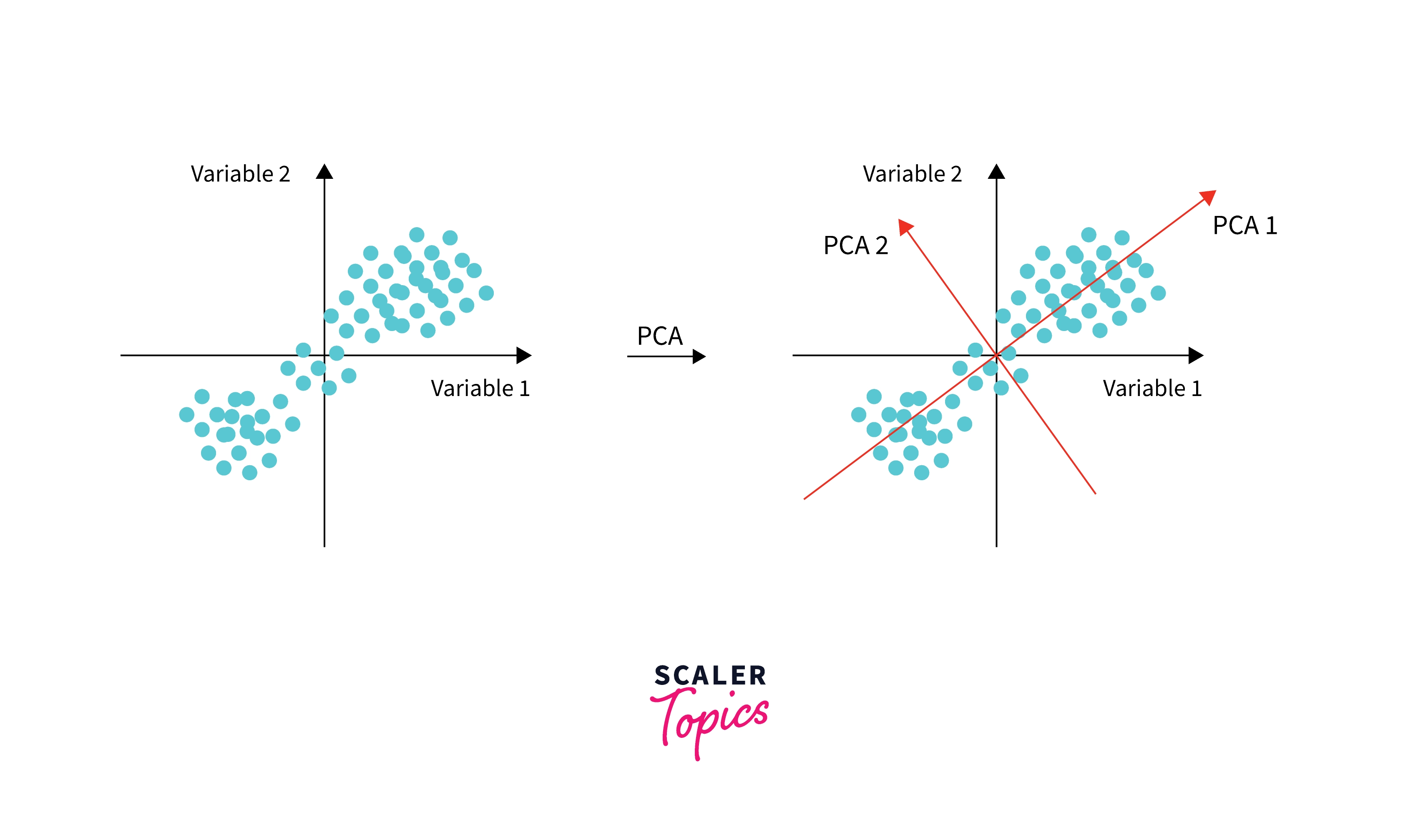
By using just the first few principal components, we can often represent the vast majority of the information in the original dataset, making it much easier to visualize, analyze, and use in subsequent modeling.
Applying PCA to Lingerie Design: From Features to Dimensions
Let's ground this process in the context of your lingerie design project. The steps are methodical and build on concepts you're well-acquainted with from your statistics background.
A highly relevant parallel can be found in a study on predicting clothing sizes, which uses PCA on anthropometric data. While the goal is different, the methodology of distilling numerous body measurements into a few key shape factors is directly analogous to distilling lingerie features into style factors.
Evaluating machine learning models for clothing size prediction ...
This paper details how PCA is used on body measurement data. The process described is a standard and robust approach that we can adapt directly for our lingerie features.
Please read the subsection titled "Principal component analysis for anthropometric analysis." Pay close attention to the three stages it outlines: standardization, covariance matrix computation, and eigenvector/eigenvalue calculation.
As the paper highlights, the process is as follows:
-
Select and Measure Features: You start with your raw data. For a lingerie collection, this might include features like:
Cup_Coverage(percentage)Strap_Width(mm)Lace_Percentage(percentage)Underwire_Strength(a numeric scale)Padding_Volume(cc)Fabric_Sheerness(percentage)
-
Standardize Data: This step is critical. Features measured on different scales (e.g., millimeters vs. percentages) must be standardized (typically to have a mean of 0 and a standard deviation of 1). This ensures that features with larger numerical ranges don't disproportionately influence the analysis.
-
Compute Principal Components: The analysis is performed on the standardized data. This yields the principal components, each of which is a weighted sum of the original features. The weights are called loadings.
Interpreting the Components: Giving Meaning to the Math
The raw principal components from the calculation are optimized to explain variance, but they are not always easy to interpret. For example, PC1 might be a messy combination of positive and negative loadings from all six of our features. This is where interpretation becomes an art, aided by a technique called rotation.
The goal of rotation (the most common method being Varimax) is to "clean up" the loadings. It rotates the principal component axes in the multidimensional space to create a simpler structure where each original feature loads heavily on only one component and has small loadings on the others. This makes it much easier to identify what concept each component represents.
The following video explains how to interpret loadings and how Varimax rotation works to make them more interpretable.
PCA : how to interpret the weights/loadings and Varimax rotation
This video from TileStats provides a more technical look at interpreting PCA results, focusing on loadings and the role of Varimax rotation.
Please watch these three key parts: First, understand how loadings are calculated and what they mean from this segment. The key insight is that with standardized data, loadings are simply the Pearson correlation coefficients between the original variables and the principal components. Next, see why rotation is needed in the section from this part of the video. Finally, watch the excellent visual explanation of how Varimax rotation works to simplify the loading structure from this segment.
After rotation, you might find that:
Underwire_Strength,Padding_Volume, andCup_Coveragehave high positive loadings on PC1, while other features have loadings near zero. We could then interpret PC1 as a "Structural Support" dimension.Lace_PercentageandFabric_Sheernesshave high positive loadings on PC2. We could interpret PC2 as a "Delicate Ornamentation" dimension.
This is the essence of identifying the dominant underlying style dimensions. You transform a dozen technical measurements into 2 or 3 meaningful, interpretable concepts that describe your collection.
Numerical Exercise: Interpreting Lingerie Style Dimensions
Now, let's put this into practice. Imagine you've analyzed 50 lingerie pieces from your trend research, measuring four key features. After standardizing the data, you ran a PCA with Varimax rotation and obtained the following loading matrix for the first two principal components.
Rotated Component Loadings:
| Feature | Component 1 | Component 2 |
|---|---|---|
Strap_Width |
0.89 | 0.12 |
Padding_Volume |
0.92 | -0.05 |
Lace_Coverage |
0.08 | 0.95 |
Fabric_Sheerness |
-0.15 | 0.85 |
Your task is to interpret these results.
- For each component, identify the original features that "load" heavily on it. A common rule of thumb is to consider loadings with an absolute value greater than 0.7 as significant.
- Based on the features you identified, propose a descriptive name for Component 1 and Component 2 that captures their essence in lingerie design terms.
- Describe in a sentence what a lingerie piece with a high positive score on Component 1 would be like.
- Describe in a sentence what a lingerie piece with a high positive score on Component 2 would be like.
Take a few minutes to analyze the table and formulate your answers.
Click to see the detailed solution.
Here is a step-by-step interpretation of the PCA results:
-
Identify Significant Loadings:
- Component 1:
Strap_Width(0.89) andPadding_Volume(0.92) have high positive loadings. The other loadings are small. - Component 2:
Lace_Coverage(0.95) andFabric_Sheerness(0.85) have high positive loadings. The other loadings are small.
- Component 1:
-
Name the Components:
- Component 1: "Structural Support" or "Substance". This component is defined by features that add physical structure, shape, and support to a garment. High values on these features correspond to more robust, shaping pieces.
- Component 2: "Delicacy & Ornamentation" or "Sheer Romance". This component is defined by features associated with lightness, transparency, and decorative elements. High values correspond to more ethereal, delicate, and less functional pieces.
-
Describe a High Score on Component 1:
A lingerie piece with a high positive score on Component 1 would be highly structured, likely featuring wide straps and significant padding, such as a robust push-up or a supportive full-cup bra. -
Describe a High Score on Component 2:
A lingerie piece with a high positive score on Component 2 would be very delicate and decorative, characterized by extensive lace and sheer fabrics, like a non-wired bralette or a transparent babydoll.
By performing this analysis, you have successfully reduced four specific measurements into two meaningful, high-level style dimensions that are much easier to think about and design with.
Conclusion
In this lesson, we introduced Principal Component Analysis as a powerful method for navigating the complexity of multivariate data. You've seen how PCA works conceptually to find the axes of greatest variation and how it can be practically applied to a lingerie dataset to achieve dimensionality reduction. Most importantly, you've learned the critical step of using rotated loadings to interpret these abstract components and assign them meaningful names that are relevant to your design work.
Key Takeaways:
- PCA reduces a large set of correlated features into a smaller set of uncorrelated Principal Components.
- Each PC captures a portion of the total variance in the data, with PC1 capturing the most.
- Loadings represent the correlation between the original features and the new components, telling us how each feature contributes to the component.
- Varimax rotation simplifies the loading structure, making it possible to interpret and name the components as underlying "style dimensions" (e.g., 'Structure' vs. 'Delicacy').
In our next lesson, we will continue this topic by focusing on two crucial diagnostic tools for PCA. We will explore how to use scree plots to decide exactly how many principal components are needed to represent your data accurately, and we'll look more closely at how to visualize and interpret loading plots to deepen your understanding of the results.
