Pearson vs. Spearman: Non-Linear Relationships

Welcome to the final lesson of this module. In our last session, we ventured into survival analysis to model the lifespan of a lingerie trend. We now return to the theme of correlation to solidify your understanding of two key measures. Having been introduced to both Pearson and Spearman correlation in earlier lessons, today we will put them head-to-head in a practical application.

This lesson is designed to address a crucial challenge in data analysis: choosing the right tool for the job. You will solve a numerical problem that directly compares Pearson and Spearman correlation on a dataset with a non-linear relationship. This exercise will reinforce why simply running a standard correlation test can be misleading and how Spearman's rank correlation can reveal strong relationships that Pearson's method might underestimate. For your goal of optimizing lingerie styles, this is vital, as the connection between a design feature and its perceived appeal is often more complex than a simple straight line.

When a Straight Line Isn't Enough: Linear vs. Monotonic Relationships

As you know from your statistical training, Pearson's correlation coefficient ( $r$ ) is the standard measure of the linear association between two continuous variables. It quantifies how well a straight line can describe the relationship. However, what happens when the relationship is consistent but not linear?

For instance, consider the relationship between fabric transparency and perceived "daringness." A small increase from 0% to 10% transparency might cause a huge jump in perceived daring. But an increase from 80% to 90% transparency might have a much smaller effect, as the garment is already considered very daring. The relationship is one of diminishing returns—it's consistently positive, but it curves.

This is where Spearman's rank correlation ( $r_{s}$ ) becomes essential. It assesses the strength of a monotonic relationship. A relationship is monotonic if, as one variable increases, the other variable consistently increases or consistently decreases, but not necessarily at a constant rate.

The following reading provides an excellent review of these concepts.

Spearman's Correlation Explained - Statistics By Jim

This article from Statistics By Jim clearly articulates the difference between the two correlation types and illustrates the scenarios where each is appropriate.

Please read the introductory section, "Choosing Between Spearman’s and Pearson’s Correlation," which uses helpful graphs to define linear and monotonic relationships. Then, skip to the section "Comparing Spearman’s and Pearson’s Coefficients" to see a direct comparison of how the two coefficients behave under different conditions.

Spearman’s correlation achieves this by a clever transformation: instead of using the raw data values, it calculates Pearson's correlation on the ranks of the data. This process effectively ignores the specific magnitudes of the changes and focuses only on the ordinal relationship between the observations.

The images below provide a powerful visual summary of this concept.

This diagram clearly shows that for linear data, Pearson and Spearman give nearly identical results. However, for non-linear but monotonic data, Pearson's coefficient (0.76) significantly underestimates the strength of the relationship, which Spearman's coefficient (0.92) captures more accurately.

These scatterplots further illustrate the point. The plot on the far right shows a perfect monotonic relationship (as X increases, Y always increases). Spearman correlation is 1, indicating a perfect monotonic trend. Pearson correlation is lower (0.88) because the relationship is not perfectly linear.

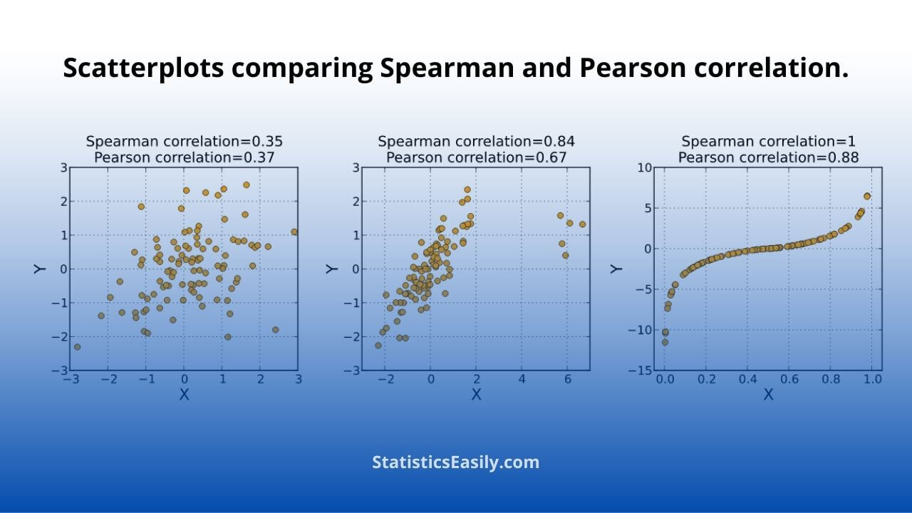
To see how the calculation on ranks works and to review the key differences between the two methods, the following video provides a concise summary.

Spearman's rank correlation | Pearson VS Spearman

This video from TileStats offers a clear, side-by-side comparison of the properties of Pearson and Spearman correlation.

Please watch the segment from the comparison. Focus on the discussion of data scale (continuous vs. ordinal), the type of relationship evaluated (linear vs. monotonic), and sensitivity to outliers.

Numerical Exercise: Strap Complexity vs. Aesthetic Appeal

Now, let's apply these concepts to a concrete design problem. Imagine you are experimenting with a new harness-style bra. You create 8 prototypes, each with an increasing number of decorative straps. You ask a professional stylist to rate the "aesthetic appeal" of each prototype on a 10-point scale.

Here is the data you collected:

Prototype ID	Strap Complexity (X)	Aesthetic Appeal (Y)
1	1	2.5
2	2	4.0
3	3	5.0
4	4	6.5
5	5	7.5
6	6	8.0
7	7	8.2
8	8	8.3

A quick glance at the data (and a mental scatterplot) suggests that while appeal generally increases with complexity, the effect seems to level off. This points towards a non-linear, monotonic relationship.

Your Task:

Calculate Pearson's correlation coefficient ( $r$ ) for this dataset.
Rank the data for both variables, Strap Complexity and Aesthetic Appeal.
Calculate Spearman's rank correlation coefficient ( $r_{s}$ ) by computing Pearson's correlation on the ranks.
Compare and interpret the two coefficients. Which is a more appropriate measure for this relationship, and why?

Please take your time to perform the calculations. You will need the formula for Pearson's correlation, which you can apply to the raw data for part 1 and the ranked data for part 3.

$r = \frac{\sum ( x _{i} - x ˉ ) ( y _{i} - y ˉ )}{\sum ( x _{i} - x ˉ ) ^{2} \sum ( y _{i} - y ˉ ) ^{2}}$

Click to see the detailed solution.

Let's break down the solution step-by-step.

1. Calculate Pearson's Correlation Coefficient ( $r$ )

First, we need the means of X and Y.
$x ˉ = (1 + 2 + 3 + 4 + 5 + 6 + 7 + 8) /8 = 36/8 = 4.5$
$y ˉ = (2.5 + 4.0 + 5.0 + 6.5 + 7.5 + 8.0 + 8.2 + 8.3) /8 = 50/8 = 6.25$

Next, we build a table for the intermediate calculations:

X	Y	$x_{i} - x ˉ$	$y_{i} - y ˉ$	$(x_{i} - x ˉ) (y_{i} - y ˉ)$	$(x_{i} - x ˉ)^{2}$	$(y_{i} - y ˉ)^{2}$
1	2.5	-3.5	-3.75	13.125	12.25	14.0625
2	4.0	-2.5	-2.25	5.625	6.25	5.0625
3	5.0	-1.5	-1.25	1.875	2.25	1.5625
4	6.5	-0.5	0.25	-0.125	0.25	0.0625
5	7.5	0.5	1.25	0.625	0.25	1.5625
6	8.0	1.5	1.75	2.625	2.25	3.0625
7	8.2	2.5	1.95	4.875	6.25	3.8025
8	8.3	3.5	2.05	7.175	12.25	4.2025
Sum				35.80	42.0	33.38

Now, we plug the sums into the formula:
$r = \frac{35.80}{42.0 \times 33.38} = \frac{35.80}{1401.96} = \frac{35.80}{37.44} \approx 0.956$

So, Pearson's $r \approx 0.956$ . This indicates a very strong positive linear relationship.

2. Rank the Data

Now we rank both variables from 1 (lowest) to 8 (highest). Since there are no ties, the ranking is straightforward.

X	Y	Rank(X)	Rank(Y)
1	2.5	1	1
2	4.0	2	2
3	5.0	3	3
4	6.5	4	4
5	7.5	5	5
6	8.0	6	6
7	8.2	7	7
8	8.3	8	8

3. Calculate Spearman's Correlation Coefficient ( $r_{s}$ )

We calculate Pearson's correlation on the ranks.
Let $R_{x}$ be Rank(X) and $R_{y}$ be Rank(Y). In this special case, the ranks are identical.
$R_{x} ˉ = R_{y} ˉ = (1 + 2 + ... + 8) /8 = 4.5$

The deviations $(R_{x i} - R_{x} ˉ)$ and $(R_{y i} - R_{y} ˉ)$ will be identical. The sum of squared deviations for ranks from 1 to n is given by $(n^{3} - n) /12$ . For n=8, this is $(8^{3} - 8) /12 = (512 - 8) /12 = 42$ .

So, $\sum (R_{x i} - R_{x} ˉ)^{2} = 42$ and $\sum (R_{y i} - R_{y} ˉ)^{2} = 42$ .
Since $R_{x i} = R_{y i}$ for all i, the numerator is $\sum (R_{x i} - R_{x} ˉ) (R_{y i} - R_{y} ˉ) = \sum (R_{x i} - R_{x} ˉ)^{2} = 42$ .

$r_{s} = \frac{42}{42 \times 42} = \frac{42}{42} = 1$

So, Spearman's $r_{s} = 1.0$ .

4. Compare and Interpret

Pearson's $r \approx 0.956$
Spearman's $r_{s} = 1.0$

Both coefficients indicate a very strong positive relationship. However, Spearman's coefficient is a perfect 1.0, while Pearson's is slightly less.

Interpretation: The Spearman's $r_{s} = 1.0$ tells us that the relationship is perfectly monotonic. Every time strap complexity increases, aesthetic appeal also increases, without exception. The ranks of X and Y are perfectly aligned.

The Pearson's $r \approx 0.956$ , while very high, is not 1.0. This is because the data points do not fall on a perfect straight line. The rate of increase in appeal slows down as complexity gets higher, introducing a curve. Pearson's coefficient is "penalized" for this deviation from linearity.

Conclusion: For this dataset, Spearman's rank correlation is the more appropriate and descriptive measure. It perfectly captures the flawless "more complexity, more appeal" trend in the data, whereas Pearson's, while still indicating a strong relationship, fails to capture its perfect consistency due to the non-linear nature.

Conclusion

This lesson brought together your prior knowledge of Pearson and Spearman correlation to highlight their distinct applications. By working through a concrete numerical problem, you've seen firsthand how Pearson's coefficient can underestimate the strength of a non-linear but monotonic relationship, while Spearman's coefficient accurately reflects the consistency of the trend. This is a critical distinction in your work, where aesthetic relationships are rarely simple straight lines.

Key Takeaways:

Pearson's $r$ measures the strength and direction of a linear relationship.
Spearman's $r_{s}$ measures the strength and direction of a monotonic relationship by applying the Pearson formula to ranked data.
For a relationship that is monotonic but not linear (e.g., showing diminishing returns), $r_{s}$ will typically be closer to -1 or +1 than $r$ , providing a more accurate assessment of the association's strength.
Always visualize your data with a scatterplot before calculating correlation to inform your choice of method.

This concludes our module on identifying trends and style relationships. We have covered methods for measuring linear and monotonic associations, assessing inter-rater agreement, and modeling trend lifespans.

In our next module, we will shift gears from analyzing relationships between pairs of variables to exploring the underlying structure of a dataset with many variables. We will begin with a powerful dimensionality reduction technique: Principal Component Analysis (PCA). This will allow you to distill complex feature sets—like the many attributes of a lingerie collection—into a few fundamental "style dimensions."

Recommended resources

When a Straight Line Isn't Enough: Linear vs. Monotonic Relationships

Numerical Exercise: Strap Complexity vs. Aesthetic Appeal

Conclusion