Lingerie Trend Lifespan: Exponential Modeling

Welcome to our next lesson. In our previous session, we focused on measuring agreement at a single point in time with Kendall's W, allowing you to check if your creative team shares a unified vision. We now shift our focus from a static snapshot of preferences to a dynamic view of how those preferences evolve over time. Fashion is transient, and understanding the lifecycle of a trend is a key part of trend analysis.

This lesson introduces you to the fundamentals of survival analysis, a set of statistical methods for modeling "time-to-event" data. You will learn how to model the lifespan of a lingerie trend using the exponential distribution, a foundational tool in this field. By the end of our session, you will be able to compute and interpret a trend's survival function and hazard rate, giving you a quantitative framework for predicting how long a particular style might remain in vogue.

From Static Ranks to Dynamic Lifespans: An Introduction to Survival Analysis

Survival analysis is a powerful branch of statistics used across many fields, from medicine (time until patient recovery) to engineering (time until equipment failure). In your context, we can adapt it to model the "lifetime" of a lingerie trend.

The key concepts are:

Event: A well-defined occurrence of interest. For us, this will be a trend "dying," meaning it loses its popularity or relevance for your high-end photoshoots.
Survival Time ( $T$ ): The time from the beginning of an observation period until the event occurs. This is the duration a lingerie trend remains popular.
Censoring: In many studies, the event has not yet occurred for some subjects by the end of the observation period. While we won't delve deeply into censoring today, it's a core concept in survival analysis that you've likely encountered in your studies.

Two functions are central to describing survival time distributions.

[PDF] Survival Analysis - NJIT

This document from NJIT provides a concise, formal introduction to the key functions in survival analysis, which will be familiar from your background in stochastic processes.

Please read the "Review of Last lecture" sections on the first page. Focus on the definitions of the survival random variable and the functions that characterize it, and then the implications of the survival and hazard functions.

As the reading highlights, the two most important functions for our purpose are:

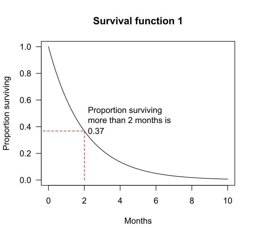
The Survival Function, $S (t)$ : This function gives the probability that the survival time $T$ is greater than or equal to some specified time $t$ .
$S (t) = P (T \geq t)$
In our lingerie project, $S (t)$ is the probability that a trend (e.g., the "cut-out" bodysuit) is still considered fashionable after time $t$ (e.g., 18 months). A high value of $S (t)$ means the trend is likely to still be viable at that future time.

This graph shows a typical survival function. It starts at 1 (100% survival at time 0) and decreases over time. The red dotted line shows that at 2 months, the probability of survival is 0.37, meaning 37% of the items are still "surviving."

The Hazard Function, $h (t)$ or $λ (t)$ : This function represents the instantaneous potential for the event to occur at time $t$ , given that it has not occurred yet.
$h (t) = lim_{Δ t \to 0} \frac{P ( t \leq T < t + Δ t ∣ T \geq t )}{Δ t}$
For our project, the hazard function represents the risk that a trend will become "unfashionable" in the very next instant, given it's popular right now. A high hazard means the trend is on shaky ground, while a low hazard suggests stability.

The Exponential Distribution: Modeling "Sudden Death" Trends

The simplest way to model survival time is with the exponential distribution. You'll recall from your operations research studies that this distribution is intrinsically linked to the Poisson process. It's used to model the time between events that occur randomly and independently at a constant average rate.

The defining feature of the exponential distribution is its constant hazard rate. This means $h (t) = λ$ for all $t > 0$ . This implies that the risk of the event occurring is the same at any point in time, regardless of how long the item has already survived. This is known as the memoryless property.

In the context of lingerie trends, this is a very strong assumption. It implies that a trend that has been popular for three years has the same risk of dying out in the next month as a trend that is only three months old. This model is most appropriate for trends that end not due to "aging" or gradual fatigue, but due to sudden, unpredictable shifts in fashion tastes—like a lightning strike.

The following resources detail the mathematical properties of the exponential distribution in a survival context.

Survival Models

This document provides a clear, narrative-driven explanation of how the exponential distribution arises from the assumption of a constant hazard.

In the PDF, find section 7.1.2, "The Hazard Function." Read the short example on the exponential distribution on page 3. It shows how the survival function S(t) = \exp(-\lambda t) is a direct consequence of the constant hazard rate \lambda.

[PDF] Survival Analysis - NJIT

This document provides the formal definitions and discusses the memoryless property, which is the key feature of the exponential model.

Now, please read the section titled "The Exponential" on page 23 of the PDF. Pay close attention to the formulas for the survival function (sf), PDF (f), and hazard function (hf), as well as the explanation of the memoryless property and its implications.

From these readings, the key formulas for the exponential distribution with rate parameter $λ$ are:

Probability Density Function (PDF): $f (t) = λ e^{- λ t}$
Survival Function: $S (t) = e^{- λ t}$
Hazard Function: $h (t) = λ$
Mean Survival Time: $E [T] = 1/ λ$

The image below visualizes these functions.

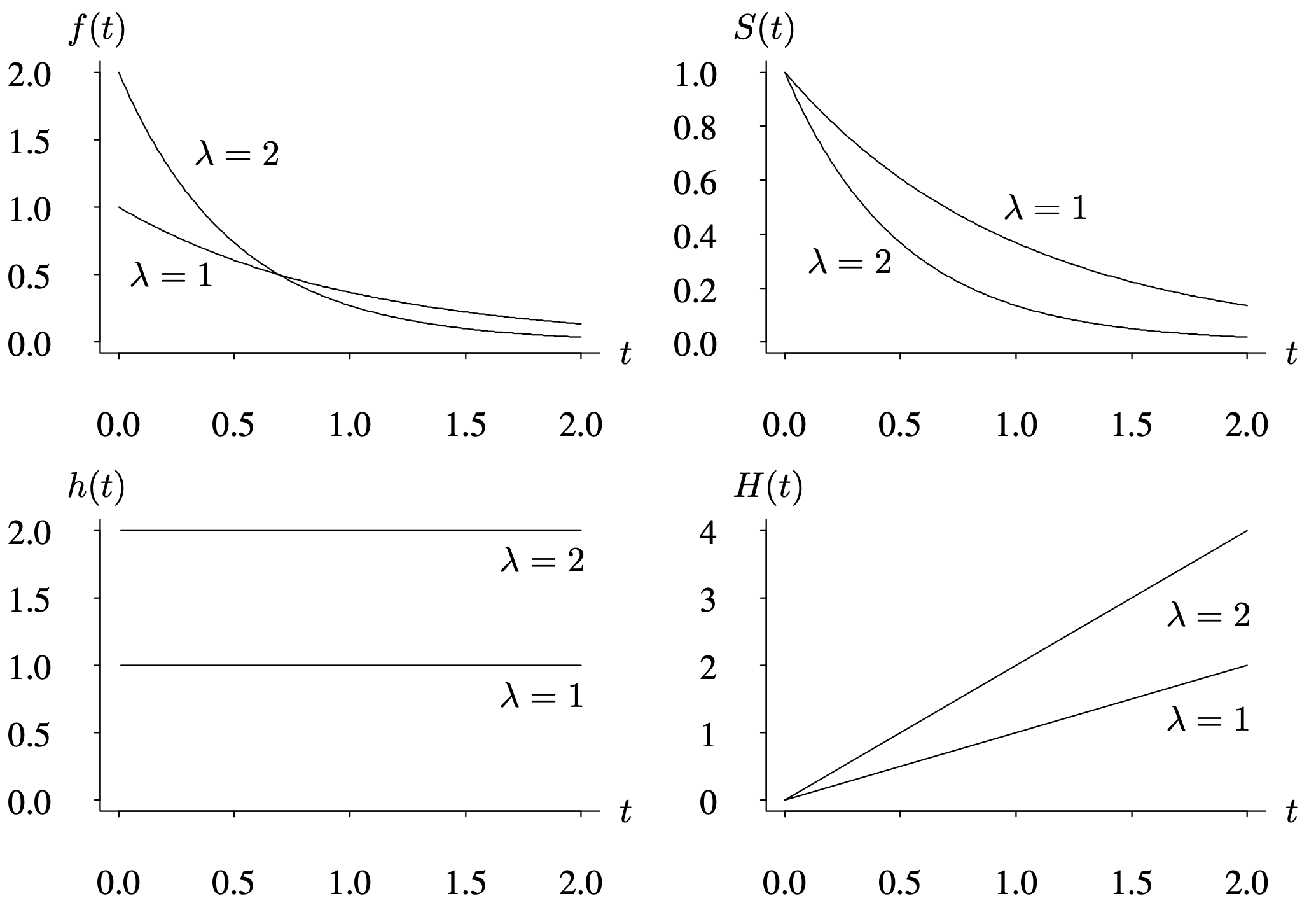
These four plots show the key functions for an exponential distribution with two different rate parameters, $\lambda=1$ and $\lambda=2$. Top-left: The Probability Density Function $f(t)$. Top-right: The Survival Function $S(t)$. Bottom-left: The constant Hazard Function $h(t)$. Bottom-right: The linear Cumulative Hazard Function $H(t)$.

Notice in the bottom-left plot how the hazard function $h (t)$ is a flat line, confirming the constant risk over time. The top-right plot shows the corresponding exponential decay of the survival probability. A higher $λ$ (like $λ = 2$ ) means a higher constant risk, which in turn leads to a faster decay in survival probability.

Numerical Exercise: Modeling the Lifespan of the "Corset Top" Trend

Let's apply this to a concrete scenario. Based on your analysis of fashion archives, you estimate that the average lifespan of a mainstream lingerie trend, like the recent popularity of the "corset top" as outerwear, is approximately 30 months. You decide to model this lifespan using an exponential distribution.

Your Task:

Calculate the rate parameter $λ$ for this distribution.
Write down the survival function $S (t)$ and the hazard function $h (t)$ for this trend.
What is the probability that the corset top trend will still be popular 12 months from now?
What is the probability that the trend will last for at least 4 years (48 months)?
Suppose the corset top trend has already been popular for 12 months. What is the probability that it survives for at least another 12 months?

Take some time to work through the calculations based on the formulas we've discussed.

Click to see the detailed solution.

1. Calculate the rate parameter $λ$ .
The mean survival time for an exponential distribution is $1/ λ$ .
We are given that the mean lifespan is 30 months.
$\frac{1}{λ} = 30$
$λ = \frac{1}{30} \approx 0.0333$
The rate parameter $λ$ is 1/30 events (trends ending) per month.

2. Write down the survival function $S (t)$ and the hazard function $h (t)$ .
Using the value of $λ$ :

Survival Function: $S (t) = e^{- t /30}$
Hazard Function: $h (t) = λ = 1/30$

3. What is the probability that the corset top trend will still be popular 12 months from now?
We need to calculate $S (12)$ .
$S (12) = e^{- 12/30} = e^{- 0.4} \approx 0.6703$
There is approximately a 67% chance that the trend will still be popular after 12 months.

4. What is the probability that the trend will last for at least 4 years (48 months)?
We need to calculate $S (48)$ .
$S (48) = e^{- 48/30} = e^{- 1.6} \approx 0.2019$
There is approximately a 20% chance that the trend will last for 4 years or more.

5. Suppose the trend has already been popular for 12 months. What is the probability that it survives for at least another 12 months?
This question tests the memoryless property. The probability of surviving an additional $z$ units of time, given survival up to time $x$ , is the same as the initial probability of surviving $z$ units of time.
$P (T \geq x + z ∣ T \geq x) = P (T \geq z) = S (z)$
In our case, $x = 12$ and $z = 12$ . We want to find $P (T \geq 24 ∣ T \geq 12)$ .
Due to the memoryless property, this is simply $S (12)$ .
$S (12) = e^{- 12/30} \approx 0.6703$
The probability is the same as the probability of surviving the first 12 months. The trend's past popularity gives it no extra momentum.

Conclusion

In this lesson, we have moved from static analysis to dynamic modeling. You've learned how to frame the lifespan of a fashion trend using the core concepts of survival analysis and applied the exponential distribution as a first-pass model. While its memoryless property is a strong and often unrealistic assumption, it provides a crucial baseline for understanding more complex survival models (like the Weibull or Cox proportional hazards models) that you may explore in the future.

Key Takeaways:

Survival Analysis provides tools to model time-to-event data, which can be adapted to analyze the lifespan of fashion trends.
The Survival Function $S (t)$ gives the probability of a trend remaining popular beyond time $t$ .
The Hazard Function $h (t)$ measures the instantaneous risk of a trend becoming unpopular at time $t$ .
The Exponential Distribution models survival with a constant hazard rate ( $λ$ ), implying a memoryless property: the future lifespan of a trend is independent of its past duration.

In the previous lessons, we've explored different ways to measure relationships and trends. Our next lesson will circle back to correlation, where you will tackle a numerical problem that directly compares Pearson and Spearman correlation, reinforcing your understanding of when to use each method, particularly when dealing with non-linear relationships between design attributes and photoshoot appeal.

Recommended resources

From Static Ranks to Dynamic Lifespans: An Introduction to Survival Analysis

The Exponential Distribution: Modeling "Sudden Death" Trends

Numerical Exercise: Modeling the Lifespan of the "Corset Top" Trend

Conclusion