Welcome back. In our previous two lessons on Principal Component Analysis, we developed a powerful method for boiling down a large number of lingerie design features into a few core, interpretable "style dimensions," such as "Coverage vs. Reveal" or "Visual Pop." You learned how to decide how many of these dimensions to keep and how to give them meaningful names.
Now, we will put those dimensions to practical use. Knowing the underlying axes of style is one thing; using them to automatically group similar items is another. Today's lesson introduces you to agglomerative hierarchical clustering, an unsupervised learning technique perfect for discovering natural "style families" within your lingerie collection. We will focus on the mechanics of how this bottom-up clustering works and, crucially, how different choices in the algorithm's setup can lead to very different groupings.
By the end of this lesson, you will be able to perform this type of clustering and compare the results of single-linkage and complete-linkage methods by interpreting their respective tree-like diagrams, called dendrograms.
The Logic of Agglomerative Clustering
Imagine laying out every lingerie piece from your collection on a large table. The goal is to group them into piles of similar styles. Agglomerative clustering automates this process in a structured, bottom-up fashion.
The algorithm is quite intuitive:
- Initialize: Start by treating each individual lingerie piece as its own cluster. If you have 50 pieces, you start with 50 clusters.
- Merge: Find the two closest clusters and merge them into a single new cluster.
- Update: Recalculate the distances between this new cluster and all other remaining clusters.
- Repeat: Continue repeating steps 2 and 3 until all pieces have been merged into one giant cluster.
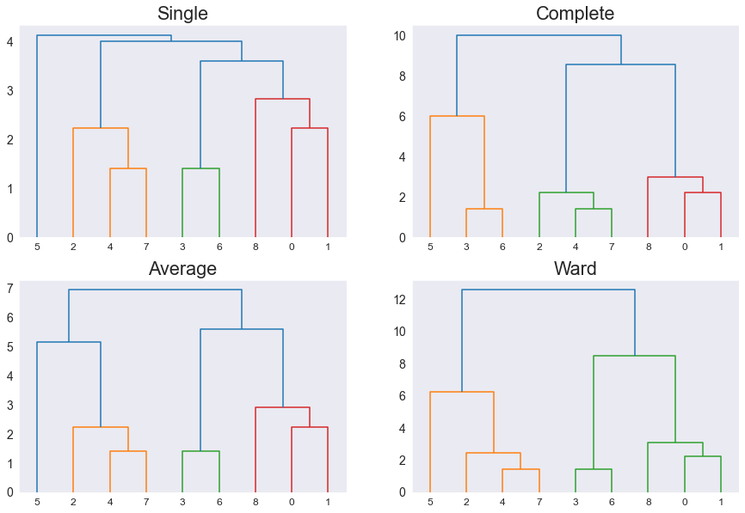
This entire process creates a hierarchy of clusters, from the most specific (single items) to the most general (all items). The visual representation of this hierarchy is a dendrogram. The y-axis of a dendrogram represents the distance or "dissimilarity" at which merges occur. Longer vertical lines signify that two more dissimilar groups are being merged.
For a thorough grounding in the algorithm and its concepts, the following guide is an excellent resource.
Hierarchical Clustering: Complete Guide with Dendrograms ...
This guide provides a clear and comprehensive explanation of hierarchical clustering. It begins by situating the method within unsupervised learning and then details the step-by-step process of the agglomerative algorithm.
Please read the introduction, Hierarchical Clustering, to get a general overview. Then, proceed to the section "Building the Hierarchy," paying close attention to the six steps that describe how the hierarchy is built from the bottom up.
Measuring Distance Between Clusters: The Role of Linkage
The most critical part of the algorithm is Step 3: updating distances. Measuring the distance between two individual lingerie pieces is straightforward (e.g., Euclidean distance based on their PCA scores). But how do you measure the distance between two clusters, each containing multiple pieces?
This is determined by the linkage criterion. The choice of linkage criterion fundamentally dictates the shape and nature of the clusters that are formed. For this lesson, we will focus on two opposing criteria: single linkage and complete linkage.
Single Linkage: The Optimist's Rule
Single linkage defines the distance between two clusters as the distance between their two closest members. It asks: "What is the shortest possible bridge between these two groups of lingerie?"
- Behavior: This criterion is "optimistic" and easily connects clusters. It is effective at identifying non-elliptical or elongated shapes (e.g., a "continuum of minimalism" from simple bralettes to slightly more structured ones).
- Drawback: It's susceptible to a phenomenon called "chaining," where a few intermediate points can cause two otherwise distinct clusters to be merged. It can be sensitive to noise.
Complete Linkage: The Pessimist's Rule
Complete linkage defines the distance between two clusters as the distance between their two farthest members. It asks: "What is the longest gap we would have to cross to connect these two groups?"
- Behavior: This criterion is "pessimistic" or strict. It will only merge clusters if all items in the resulting new cluster are relatively close to one another. This tends to produce tight, compact, roughly spherical clusters.
- Drawback: It can have trouble with non-globular clusters and may break up natural, elongated groupings that single linkage would have found.
The following video provides an excellent visual and conceptual explanation of these two linkage methods.
IAML19.5 Single-link, complete-link, Ward's method
This video from Victor Lavrenko's machine learning course clearly contrasts single-linkage and complete-linkage clustering.
Watch the section on single linkage, which explains the minimum-distance criterion. Then, watch the section on complete linkage, which explains the maximum-distance criterion and how it leads to more compact, spherical clusters.
To solidify your understanding of these critical differences, please read the following section from the guide we consulted earlier.
Hierarchical Clustering: Complete Guide with Dendrograms ...
This section succinctly defines and contrasts single, complete, and average linkage.
Focus on the subsections Single Linkage and Complete Linkage. Notice the emphasis on how single linkage finds connections while complete linkage enforces compactness.
Visualizing the Impact of Linkage
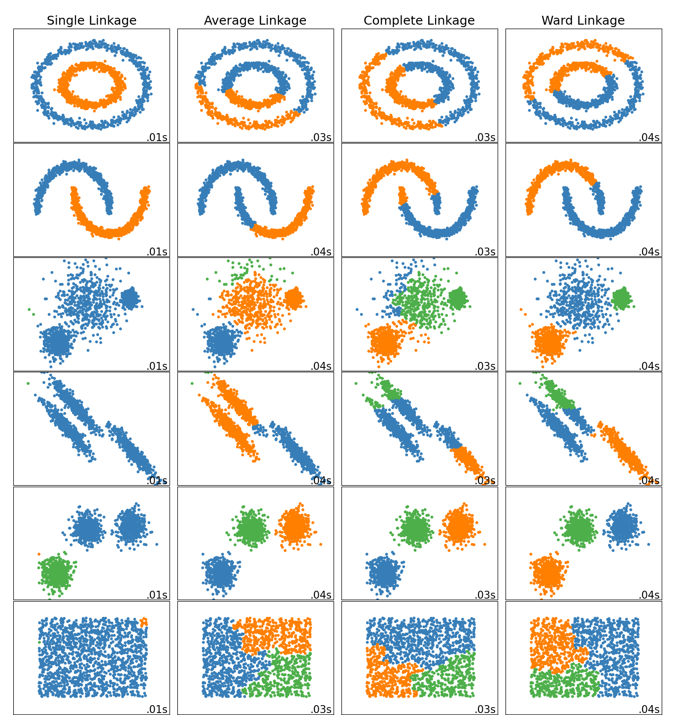
The choice of linkage has a dramatic effect on the final clustering. The image below shows how different linkage methods perform on various 2D datasets. Pay attention to the first column (Single Linkage) and third column (Complete Linkage).
This difference in behavior is also directly reflected in the structure of the dendrogram.
A Worked Example: Clustering Lingerie Styles
Given your background, let's walk through a concrete numerical example. Suppose we've run PCA on a set of lingerie features and retained two components: PC1 ("Delicacy") and PC2 ("Structure"). We have five lingerie pieces with the following scores:
| Piece | Style Description | PC1 (Delicacy) | PC2 (Structure) |
|---|---|---|---|
| 1 | Lace Bralette | 0.9 | 0.1 |
| 2 | Silk Robe | 0.8 | 0.2 |
| 3 | Padded Push-up Bra | 0.1 | 0.9 |
| 4 | Underwire Balconette | 0.2 | 0.8 |
| 5 | Strappy Garter Belt | 0.5 | 0.5 |
The step-by-step manual calculation of hierarchical clustering can be quite illuminating. The following resource provides an excellent template for this.
The complete guide to clustering analysis: k-means and hierarchical ...
This guide provides an exceptional by-hand walkthrough of hierarchical clustering. We will follow its structure to see how the linkage choice impacts our lingerie example.
First, review how the initial distance matrix is computed in the section Solution by hand. Then, carefully follow the step-by-step logic for Single linkage and Complete linkage. The key is to see how the distance matrix is updated differently after each merge.
Let's apply this logic to our lingerie data.
1. Initial Distance Matrix
First, we calculate the Euclidean distance between all pairs of points. For example, the distance between Piece 1 (Lace Bralette) and Piece 3 (Padded Push-up Bra) is:
The full initial distance matrix is:
| 1 | 2 | 3 | 4 | 5 | |
|---|---|---|---|---|---|
| 1 | 0 | ||||
| 2 | 0.14 | 0 | |||
| 3 | 1.13 | 1.06 | 0 | ||
| 4 | 0.99 | 0.92 | 0.14 | 0 | |
| 5 | 0.57 | 0.42 | 0.57 | 0.42 | 0 |
2. First Merge (Same for Both Methods)
The smallest distance is 0.14, which occurs twice. Let's merge Piece 1 (Lace Bralette) and Piece 2 (Silk Robe). Our clusters are now: {1,2}, {3}, {4}, {5}.
3. Second Merge & Divergence
Here's where the methods diverge. We need to find the next smallest distance.
- The distance between
{3}and{4}is still 0.14. - We must now calculate the distances from our new cluster
{1,2}to all others.
Single Linkage (Minimum Distance):
d({1,2}, 3) = min(d(1,3), d(2,3)) = min(1.13, 1.06) = 1.06d({1,2}, 4) = min(d(1,4), d(2,4)) = min(0.99, 0.92) = 0.92d({1,2}, 5) = min(d(1,5), d(2,5)) = min(0.57, 0.42) = 0.42
The smallest distance in our updated world isd(3,4) = 0.14. So, single linkage merges{3}and{4}next. The clusters become{1,2},{3,4},{5}. This makes intuitive sense: we have a 'delicate' cluster{1,2}and a 'structured' cluster{3,4}.
Complete Linkage (Maximum Distance):
d({1,2}, 3) = max(d(1,3), d(2,3)) = max(1.13, 1.06) = 1.13d({1,2}, 4) = max(d(1,4), d(2,4)) = max(0.99, 0.92) = 0.99d({1,2}, 5) = max(d(1,5), d(2,5)) = max(0.57, 0.42) = 0.57
The distances available for merging ared(3,4)=0.14,d({1,2},5)=0.57,d(3,5)=0.57, etc. The smallest is stilld(3,4)=0.14. So, complete linkage also merges{3}and{4}next.
In this simple case, the first two merges were the same. The differences would become more apparent in subsequent steps as the clusters grow larger. For instance, single linkage would eventually merge {5} (the Garter Belt) with the 'delicate' cluster {1,2} based on its relatively small distance of 0.42. Complete linkage, being more conservative, might merge it differently depending on the maximum distances.
This demonstrates that while the process is deterministic, the path it takes—and the final hierarchy—is entirely dependent on the linkage criterion you choose.
Numerical Exercise
Consider the following distance matrix for five bikini styles: A (String), B (Bandeau), C (High-Neck), D (Underwire), and E (Sport Top).
| A | B | C | D | E | |
|---|---|---|---|---|---|
| A | 0 | ||||
| B | 1.2 | 0 | |||
| C | 3.5 | 3.1 | 0 | ||
| D | 3.8 | 3.4 | 0.8 | 0 | |
| E | 4.1 | 3.9 | 1.1 | 0.5 | 0 |
- First Merge: Which two styles are merged first? At what distance?
- Second Merge (Single Linkage): After the first merge, which two clusters are merged next using the single linkage criterion? Show the calculation.
- Second Merge (Complete Linkage): After the first merge, which two clusters are merged next using the complete linkage criterion? Show the calculation.
Click for a detailed solution.
-
First Merge: The smallest value in the matrix is 0.5, the distance between D (Underwire) and E (Sport Top). They are merged first at a height of 0.5. The clusters are now
{A},{B},{C},{D,E}. -
Second Merge (Single Linkage): We need to find the new minimum distance. The existing distances are
d(A,B)=1.2,d(A,C)=3.5,d(B,C)=3.1. We calculate new distances to the{D,E}cluster:d(A, {D,E}) = min(d(A,D), d(A,E)) = min(3.8, 4.1) = 3.8d(B, {D,E}) = min(d(B,D), d(B,E)) = min(3.4, 3.9) = 3.4d(C, {D,E}) = min(d(C,D), d(C,E)) = min(0.8, 1.1) = 0.8
The set of available distances is{1.2, 3.5, 3.1, 3.8, 3.4, 0.8}. The smallest is 0.8. Therefore, single linkage merges C (High-Neck) with the {D,E} cluster next. This forms a larger "supportive/coverage" family.
-
Second Merge (Complete Linkage): We calculate the new distances using the maximum:
d(A, {D,E}) = max(d(A,D), d(A,E)) = max(3.8, 4.1) = 4.1d(B, {D,E}) = max(d(B,D), d(B,E)) = max(3.4, 3.9) = 3.9d(C, {D,E}) = max(d(C,D), d(C,E)) = max(0.8, 1.1) = 1.1
The set of available distances is{1.2, 3.5, 3.1, 4.1, 3.9, 1.1}. The smallest is 1.1. Therefore, complete linkage merges C (High-Neck) with the {D,E} cluster next. In this case, the result was the same, but the merge distance (1.1) is higher than for single linkage (0.8), which will affect the dendrogram's shape. Hadd(A,B)=1.0been the case, complete linkage would have merged A and B, creating a different hierarchy entirely.
Conclusion
In this lesson, we have laid the groundwork for segmenting your lingerie collection into data-driven style families. You've learned how agglomerative hierarchical clustering builds a nested hierarchy of clusters from the bottom up and how this process is visualized using a dendrogram.
Key Takeaways:
- Agglomerative clustering starts with individual items and repeatedly merges the closest pair of clusters.
- The linkage criterion defines how the distance between clusters is measured and is a critical choice.
- Single linkage (minimum distance) is optimistic, finds chain-like structures, and is sensitive to noise.
- Complete linkage (maximum distance) is conservative, creates compact and tight clusters, and is more robust to outliers.
- Comparing dendrograms from different linkage methods reveals different potential structures in your data.
We have successfully built the full hierarchy. But how many clusters should you actually use? Three? Five? In our next lesson, we will address this crucial question by learning how to "cut" the dendrogram at an appropriate level to create meaningful and interpretable style segments for your lingerie project.