Vector Search for Relevant Chunks

Welcome back! In our previous lesson, we successfully populated a ChromaDB vector store, turning our processed document chunks into an indexed, searchable knowledge base. We now have the "memory" for our AI application. Today, we'll learn how to ask questions of that memory.

This lesson focuses on the heart of the "Retrieval" in Retrieval-Augmented Generation. You will learn how to perform a similarity search on your vector store to find the most relevant document chunks for any given query. This is the crucial step that connects a user's question to the specific knowledge stored in your database, setting the stage for generating an informed answer.

How Similarity Search Works

Before we write any code, let's establish a clear mental model of the retrieval process. When you query a vector store, a few things happen in sequence:

Query Embedding: Your query, which is just a text string (e.g., "What are the key features of the new iPhone?"), is converted into a vector embedding. This is done using the exact same embedding model that you used to create the embeddings for your documents. This ensures that the query and the documents exist in the same "semantic space."
Vector Comparison: The vector store then takes your new query vector and compares it to all the document vectors it has stored. This comparison is done using a mathematical distance metric.
Nearest Neighbor Search: The goal is to find the "k" nearest neighbors—the document vectors that are "closest" to your query vector according to the chosen metric. These closest documents are considered the most semantically relevant.

The diagram below illustrates this entire flow, from the initial data ingestion we've already done to the query and retrieval process we're focusing on now.

This diagram shows the end-to-end RAG workflow. We are now implementing the top path: a User Query is converted into an embedding and used for a Semantic Search against the HNSW Index within ChromaDB to retrieve relevant context.

Choosing and Understanding Similarity Metrics

The notion of "closeness" is defined by a similarity metric. In our last lesson, we configured our ChromaDB collection with metadata={"hnsw:space": "cosine"}. This tells the underlying HNSW index to use cosine similarity to measure the proximity between vectors.

While cosine similarity is extremely common, especially for text, other metrics exist. Each measures "closeness" in a slightly different way.

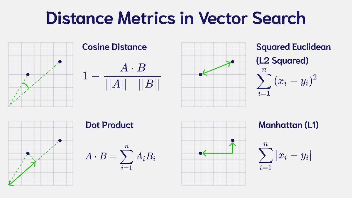
This image displays four common distance metrics: Cosine Distance, Squared Euclidean (L2), Dot Product, and Manhattan (L1). Notice that Cosine Distance focuses on the angle between vectors, whereas L2 and L1 focus on the spatial distance between their endpoints.

The most important principle when choosing a metric is consistency.

Similarity Metrics for Vector Search

This article from the Zilliz blog clearly explains the guiding principle for metric selection.

Please read the section titled The Principle of Metric Selection. The key takeaway is the rule of thumb: match the similarity metric in your vector store to the one used to train the embedding model.

For many popular sentence-transformer models, like the all-MiniLM-L6-v2 we've been using, cosine similarity was used during training. Therefore, using it for retrieval ensures the most accurate results.

Performing Queries with ChromaDB

With the conceptual groundwork laid, let's move to the practical implementation. In ChromaDB, you perform a similarity search using the collection.query() method. It's a powerful and flexible tool for retrieving information.

The following article from Real Python, which we also used in the last lesson, provides an excellent walkthrough.

Embeddings and Vector Databases With ChromaDB

This section will guide you through the practical steps of querying your collection.

Start from the heading With documents embedded. This section demonstrates how to use collection.query() with single and multiple queries, explains the key parameters like query_texts and n_results, and shows how to interpret the dictionary of results.

Let's break down the key elements from the article. A typical query call looks like this:




# Assuming 'collection' is your populated ChromaDB collection object

query_results = collection.query(
    query_texts=["Find me some delicious food!"], # The text to search for
    n_results=1,                                # The number of results to return
)




# Let's inspect the results
print(query_results)

The collection.query() method returns a dictionary containing the results. The most important keys are:

'documents': A list of lists containing the text of the retrieved document chunks.
'metadatas': A list of lists containing the metadata associated with each retrieved chunk.
'distances': A list of lists containing the calculated distance for each result.
'ids': A list of lists with the unique IDs of the retrieved chunks.

It's crucial to understand the 'distances' value. When using cosine similarity, ChromaDB returns the cosine distance, which is calculated as $1 - cosine similarity$ .

A cosine similarity of 1 (identical vectors) results in a distance of 0.
A cosine similarity of -1 (opposite vectors) results in a distance of 2.

Therefore, when you search, lower distances are better. The vector store will return the items with the smallest distance values first.

Similarity vs. Distance: An Important Distinction

The concepts of "similarity" and "distance" are inversely related, and it's essential to be clear on which one you're working with. High similarity means low distance, and vice-versa. When you ask a database to retrieve results, you need to specify the correct sorting order.

This next video offers a brilliant and intuitive explanation of this distinction, using a SQL-like syntax that should resonate with your background as a software engineer. It helps to think of vector search as just another type of database query, with its own specific operators and ordering rules.

Beginner's Guide to Vector Databases

This video from the "AI by Hand" channel provides a clear, visual breakdown of similarity versus distance and shows how this translates into a database query.

First, watch from this segment to understand the visual difference between similarity (overlap) and distance (separation), and how they correspond to descending and ascending order, respectively. Next, watch from the following part, which shows a SELECT statement using DOT_PRODUCT (a similarity metric) and ORDER BY score DESC. This reinforces the idea that for similarity, you want the highest score, so you order in descending order.

To summarize the video's key point:

When retrieving by similarity (e.g., dot product), you want the highest scores first. You would order the results in DESC (descending) order.
When retrieving by distance (e.g., L2/Euclidean or cosine distance), you want the lowest scores first. You would order the results in ASC (ascending) order.

ChromaDB handles this for you automatically. When you call .query(), it finds the items with the smallest distance.

The Need for Efficient Search

Imagine your vector store contains millions of documents. If you performed a brute-force search, your query vector would need to be compared with every single document vector. As a software engineer, you can immediately see this approach doesn't scale. This is O(N) complexity, where N is the number of documents.

The video below explains this inefficient brute-force approach, which helps clarify why vector databases don't do it this way.

Beginner's Guide to Vector Databases

This final clip from the same video illustrates the problem with a brute-force K-Nearest Neighbor search.

Watch the short segment from this timestamp. It shows the process of repeatedly scanning the entire list of vectors to find the top k results.

This is precisely why vector stores use Approximate Nearest Neighbor (ANN) algorithms, like the HNSW index we discussed in the previous lesson. These algorithms build clever data structures (like graphs) that allow them to find almost the best matches very quickly, without having to check every single vector. They trade a tiny amount of perfect accuracy for a massive gain in speed, which is a classic and essential engineering trade-off.

Conclusion

In this lesson, you've learned how to harness the power of your populated vector store by performing similarity searches. You've gone from simply storing data to actively retrieving relevant information based on semantic meaning.

Here are the key takeaways:

Similarity Search Process: A query is embedded, then compared against document embeddings using a distance metric to find the nearest neighbors.
ChromaDB's query() Method: This is your primary tool for retrieval. You provide query texts and specify the number of results (n_results).
Interpreting Results: The method returns a dictionary containing the retrieved documents, their metadata, and importantly, their distances. For cosine-based search, a smaller distance signifies greater relevance.
Similarity vs. Distance: Remember that they are inversely related. High similarity corresponds to low distance. Queries are typically ordered to find the smallest distance.
Efficiency is Key: Vector databases rely on ANN indexes like HNSW to perform these searches efficiently at scale, avoiding slow, brute-force comparisons.

You now have the core retrieval mechanism in place. However, sometimes a broad similarity search isn't enough. You might want to find documents that are not only semantically similar but also meet specific criteria, like coming from a particular source file or created within a certain date range.

In our next lesson, we will explore this by learning how to apply metadata filters during retrieval to narrow down search results, giving you much more precise control over your RAG pipeline.