Populating Vector Stores with Document Chunks and Embeddings

Setting Up Your Vector Store: ChromaDB

Let's get started with ChromaDB. As a software engineer, you can think of this as setting up any new database driver or client in a project. The first step is installation.

pip install chromadb

Once installed, you need to initialize a client. ChromaDB offers a few ways to run, but for our purposes, the two most important are the in-memory and persistent modes.

• In-Memory Client (EphemeralClient): This client stores all data in memory and is wiped clean when your script finishes. It's excellent for quick tests, experiments, or temporary applications.
• Persistent Client (PersistentClient): This client saves your data to disk at a specified path. This is what you'll typically use in a project, as it allows your indexed knowledge base to persist across different sessions and application restarts.

We will use the persistent client to ensure our work is saved. The following article from Real Python provides a great hands-on guide. We'll start by setting up our environment and client.

Following the article, our initial setup in Python will look like this:

import chromadb
from chromadb.utils import embedding_functions




# Define a path for our persistent storage
CHROMA_DATA_PATH = "rag_knowledge_base"




# Create a persistent client
client = chromadb.PersistentClient(path=CHROMA_DATA_PATH)

This simple setup gives us a client object connected to a database that will be stored in the rag_knowledge_base directory.

Creating a Collection

Within ChromaDB, your data is organized into collections. A collection is the direct equivalent of a table in a relational database or a collection in MongoDB. It holds your embeddings, their associated documents (chunks), and metadata.

To create a collection, you can use client.create_collection(). A more robust method, especially in a real application, is client.get_or_create_collection(), which will create the collection if it doesn't exist or simply retrieve it if it does, preventing errors on subsequent runs.

When creating a collection, you need to define a few important parameters:

1. name: A unique name for your collection.
2. embedding_function: This is a critical choice. You are telling ChromaDB how to convert your text documents into vector embeddings. If you don't specify one, ChromaDB uses a default model. However, for control and consistency, it's best to define it explicitly.
3. metadata: This optional dictionary can be used to configure the collection. A key use case is specifying the distance metric for the underlying HNSW index, such as {"hnsw:space": "cosine"} to use cosine similarity, which we discussed in Module 2.

Let's continue with the Real Python article to see how this is done.

Here's the code to create our collection, adapted from the article:

# Define the embedding model we'll use
EMBED_MODEL = "all-MiniLM-L6-v2"
embedding_func = embedding_functions.SentenceTransformerEmbeddingFunction(
    model_name=EMBED_MODEL
)




# Define the collection name
COLLECTION_NAME = "my_documents"




# Create the collection
collection = client.get_or_create_collection(
    name=COLLECTION_NAME,
    embedding_function=embedding_func,
    metadata={"hnsw:space": "cosine"}
)

Now we have an empty but fully configured collection, ready to be populated.

Adding Documents to the Collection

This is the central step: loading our data. The collection.add() method is the primary tool for this. It takes a few key arguments as lists:

• documents: The list of text strings (your document chunks).
• ids: A list of unique string identifiers for each document. This is mandatory and allows you to update or delete specific items later.
• metadatas: An optional list of dictionaries, where each dictionary contains the metadata for the corresponding document.

When you call add(), ChromaDB performs the magic behind the scenes: for each item in the documents list, it calls the embedding_function you specified, generates the vector embedding, and then stores the document, its ID, its metadata, and the new embedding in the collection.

The following diagram shows this "Indexing" phase in action. We have already completed the "Chunking" step in a previous module. Now we are executing the "Vectorize" and "Indexing" steps by populating our ChromaDB collection.

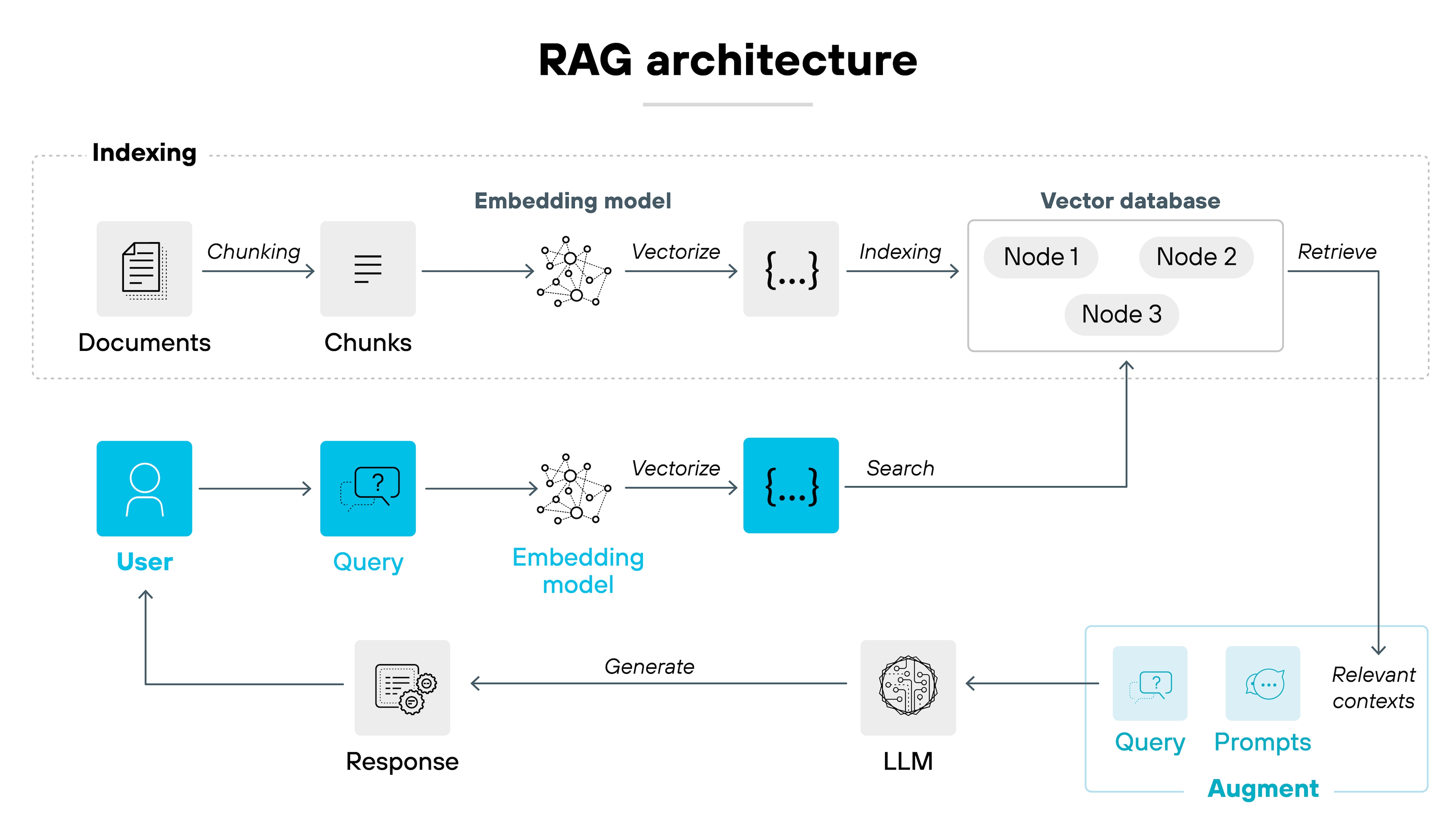
Let's see a simple, concrete example of adding a few documents.

Adapting that example, the call looks like this:

# Let's assume we have our chunks and metadata from previous lessons
chunks = [
    "The latest iPhone model comes with impressive features.",
    "Exploring the beautiful beaches and vibrant culture of Bali.",
    "Einstein's theory of relativity revolutionized our understanding of space and time."
]
metadata = [
    {"source": "apple_event.txt", "chunk_num": 1},
    {"source": "travel_blog.txt", "chunk_num": 5},
    {"source": "physics_paper.pdf", "chunk_num": 12}
]
ids = [
    "doc_001",
    "doc_002",
    "doc_003"
]




# Add the data to the collection
collection.add(
    documents=chunks,
    metadatas=metadata,
    ids=ids
)

That's it! Your three chunks are now embedded, indexed, and stored, ready to be queried.

The DataCamp article below provides another excellent walkthrough of this same process, reinforcing the concepts of client setup, collection creation, and adding documents. It also explicitly notes that Chroma will automatically download and use a default embedding model if you don't specify one.

Advanced Topic: Batching for Large Datasets

Adding a few documents is simple. But what if you have 100,000 chunks? Loading them all in a single collection.add() call might consume too much memory or hit an API limit. The standard engineering solution is batching.

We can process our documents in smaller, manageable batches. The Real Python article demonstrates a very clean way to implement this.

The core logic from that function is to iterate over your data in batches and call collection.add() for each batch. This is a much more robust and scalable pattern for populating your vector store.

Using Frameworks: The LangChain Abstraction

While it's crucial to understand the native ChromaDB API, you should also be aware that higher-level frameworks like LangChain provide convenient abstractions. For example, LangChain offers a Chroma.from_documents() class method that handles much of this process for you.

The following video by Krish Naik demonstrates how this works.

This approach is powerful for rapid development. However, by learning the underlying ChromaDB API first, you have gained the "deep knowledge" needed to customize, debug, and optimize your data ingestion pipeline effectively, which is a key goal of this course.

Conclusion

In this lesson, you have successfully bridged the gap between having processed document chunks and having a fully indexed, searchable knowledge base. You've moved from the "what" and "why" of vector stores to the practical "how."

Here are your key takeaways:

• ChromaDB Setup: You can initialize an in-memory client for testing or a persistent client to save your data to disk.
• Collections are Key: Collections are the containers for your data, analogous to tables in SQL. You create them with a name, an embedding function, and optional metadata like the distance function.
• Populating with add(): The collection.add() method is the workhorse, taking lists of documents, unique IDs, and metadata to populate the store. ChromaDB handles the embedding process internally.
• Scaling with Batching: For large datasets, adding data in batches is a crucial pattern for efficient and robust ingestion.
• Framework Abstractions: Tools like LangChain offer high-level wrappers (Chroma.from_documents) that can accelerate development, but understanding the native API is key for deeper control.

You now have a populated vector store. The final piece of the retrieval puzzle is to actually query it. In the next lesson, we will do just that: you'll learn to perform similarity search on your vector store to retrieve relevant chunks for a given query.