In our previous lessons, you've learned how to populate a vector store with document chunks and use both similarity search and metadata filters to retrieve them. We concluded by asking a crucial question for any scalable system: how can a vector database search through millions, or even billions, of vectors in milliseconds? A simple, brute-force comparison is far too slow for the real-time needs of a RAG application.
This lesson provides the answer. We will delve into the world of Approximate Nearest Neighbor (ANN) search, the core technology that makes modern vector databases fast and efficient. You will learn how these algorithms work, focusing on the most popular one, Hierarchical Navigable Small World (HNSW), and understand the fundamental trade-off it makes between search speed and perfect accuracy. This is the final piece of the puzzle for understanding the "retrieval" component of RAG.
The Problem: The Inefficiency of Perfection
Before we explore the approximation, let's first define perfection. The most straightforward way to find the nearest neighbors to a query vector is to calculate its distance to every single other vector in the database, sort the results, and return the top-k. This is known as an Exact Nearest Neighbor (KNN) or "brute-force" search.
While this method guarantees 100% accuracy—you will always find the true nearest neighbors—its computational cost scales linearly with the number of vectors, a complexity of O(N). For a software engineer, the implications are clear: if your database doubles in size, your query time also doubles. This is untenable for a production system that needs to provide real-time responses.
The video below from Redis provides an excellent primer on the fundamental difference between exact and approximate search.
Exact vs Approximate (HNSW) Nearest Neighbors in Vector Databases
This video clearly frames the problem that ANN algorithms solve.
Watch from the beginning to understand the concepts of KNN and ANN. Pay attention to the explanation of "flat" or exact search, which describes the brute-force linear scan and its scalability problem. Finally, watch the section that introduces ANN algorithms as the solution, framing them as a trade-off between precision and speed.
The Solution: Approximate Nearest Neighbor (ANN) Search
ANN algorithms operate on a simple but powerful premise: what if we could be almost perfect, but a thousand times faster? Instead of guaranteeing the absolute nearest neighbors, they aim to find vectors that are very close to the true answer, with a high probability. This trade-off is the key to their success. We sacrifice a small, often negligible, amount of accuracy for massive gains in speed and scalability, often achieving logarithmic time complexity, O(log N).
For RAG applications, this is an excellent trade-off. Retrieving documents that are 99% as relevant as the absolute best matches is almost always sufficient to provide the LLM with the necessary context. Among the many ANN algorithms, one has become the de facto standard for in-memory vector search: Hierarchical Navigable Small World (HNSW).
This article from Michael Brenndoerfer's blog provides a superb deep dive into HNSW. We will use it throughout this lesson.
To begin, read the introduction, starting from the first paragraph down to the end of the third. This section perfectly frames the problem with brute-force search and introduces HNSW as the dominant solution.
How HNSW Works: Highways and Local Roads
HNSW is a graph-based algorithm. At its core, it organizes vectors as nodes in a special kind of graph. The "magic" of HNSW comes from combining two concepts you might be familiar with from data structures and algorithms: skip lists and navigable small-world graphs.
-
Navigable Small World (NSW) Graphs: These graphs have a unique property. Most connections are short-range, linking a node to its immediate neighbors. However, they also contain a few long-range connections that act like "highways," allowing for rapid traversal across the graph. The main challenge with a simple NSW graph is that a search can get stuck in a "local minimum"—a point that seems like the best in its immediate vicinity but is far from the global best.
-
Hierarchical Structure: This is HNSW's solution to the local minimum problem. Instead of one flat graph, HNSW builds multiple layers, much like a skip list.
- The Top Layers: These are very sparse and contain only a few nodes. The connections here are long-range, acting as an express highway system across the entire vector space.
- The Bottom Layer (Layer 0): This layer is dense and contains every single vector. The connections are short-range, like a detailed map of local roads.
The search process elegantly uses this hierarchy:
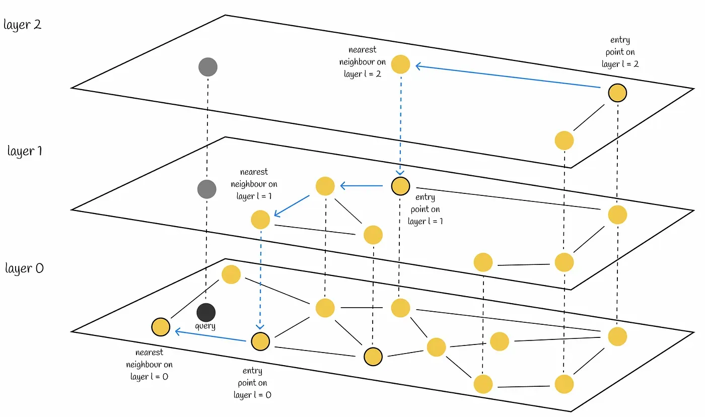
The search unfolds in two phases:
- Greedy Descent: The search starts at an entry point in the top layer. It greedily moves to the neighbor closest to the query until it can't find a closer one. It then drops down to the next layer, using its current position as the new starting point. This phase quickly "zooms in" to the correct region of the vector space.
- Fine-Grained Search: Once the search reaches the bottom layer (Layer 0), it switches to a more thorough exploration (a beam search) within that local neighborhood to identify the final set of nearest neighbors.
This two-phase process is what gives HNSW its O(log N) efficiency. You spend most of your time on the sparse upper layers, taking giant leaps across the dataset, and only perform a detailed, localized search at the very end.
This part of the article explains the core mechanics of HNSW.
First, read the section The Hierarchical Insight. This part explains the layered structure, the probabilistic assignment of nodes to layers, and how this architecture solves the local minimum problem by separating coarse and fine-grained search. Don't worry too much about the math formula for layer assignment; focus on the conceptual takeaway. Next, read the Search Procedure section. This describes the two phases—greedy descent and beam search—in detail.
Balancing Speed and Accuracy: The Tunable Knobs
The core purpose of HNSW is to balance speed and accuracy, and it provides you, the engineer, with parameters to control this trade-off. While there are a few parameters, the most important one to understand for query-time performance is ef_search.
M: The number of connections each node will have. A higherMcreates a denser graph, which can improve accuracy but uses more memory and takes longer to build.ef_construction: The size of the candidate list during index construction. A higher value creates a higher-quality graph, which leads to better search performance later, but makes the initial indexing process much slower. This is a one-time build cost.ef_search: The size of the candidate list during a search. This is the critical run-time parameter. It determines how "thorough" the search is on the bottom layer.- A low
ef_searchvalue results in a very fast query but may have lower recall (accuracy), as the search is less exhaustive. - A high
ef_searchvalue forces the algorithm to explore more potential neighbors, leading to higher recall at the cost of increased query latency.
- A low
This relationship between ef_search, query speed (often measured in queries per second, or QPS), and accuracy (recall) is the fundamental trade-off you manage when using HNSW.
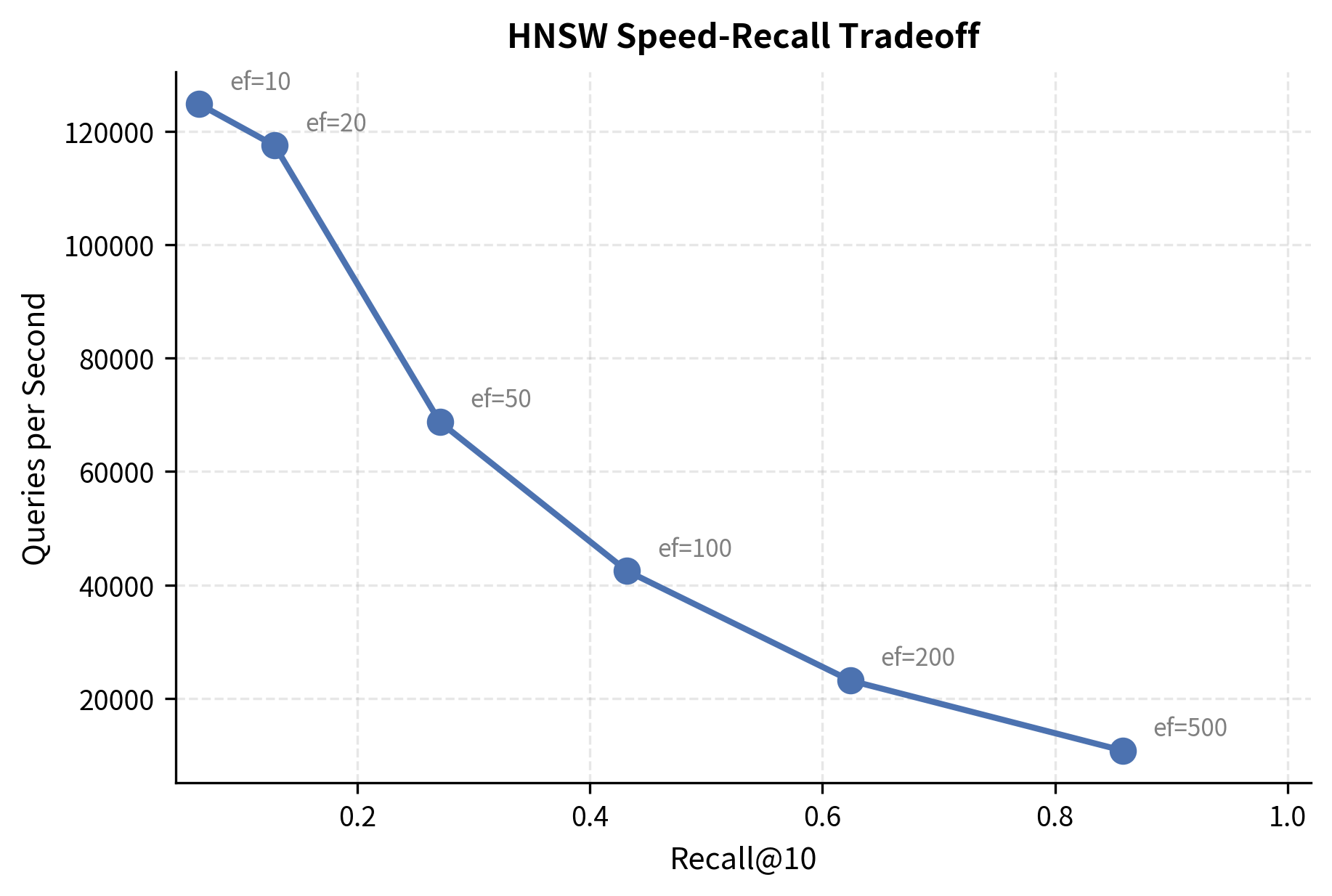
The following reading provides a fantastic summary of these parameters and demonstrates this trade-off with a practical code example.
This reading will solidify your understanding of how to control the HNSW trade-off.
First, read the section on HNSW Parameters, focusing on the descriptions of M, ef_construction, and especially ef_search. Then, jump to the section Searching with different ef_search values. Look at the table and the graph generated by the code. They perfectly illustrate how increasing ef_search improves recall while decreasing queries per second (QPS).
Conclusion
In this final lesson of the module, you've peered under the hood of modern vector databases to understand how they achieve their remarkable performance. You are now equipped with the conceptual framework to reason about the efficiency and accuracy of the retrieval step in a RAG system.
Here are the key takeaways:
- The Scalability Problem: Exact Nearest Neighbor (KNN) search is 100% accurate but scales poorly (O(N)), making it impractical for large datasets.
- The ANN Solution: Approximate Nearest Neighbor (ANN) algorithms like HNSW provide a solution by trading a small amount of accuracy for huge gains in speed, achieving O(log N) complexity.
- HNSW's Architecture: HNSW uses a hierarchical, multi-layered graph to separate search into a fast, coarse-grained "zoom-in" phase and a precise, fine-grained local search.
- The Core Trade-off: HNSW's performance is a balance between speed and recall. This trade-off is not fixed; it can be tuned at query time, primarily through the
ef_searchparameter, allowing you to tailor the system to your application's specific latency and accuracy requirements.
With this, our module on "Indexing and Retrieval" is complete. You now understand how to process documents, create embeddings, populate a vector store, and retrieve relevant information efficiently and accurately using similarity search, filters, and ANN algorithms.
In the next module, "Core RAG: Assembling the Pipeline," we will finally put all these pieces together. You will learn how to take a user's query, retrieve relevant context from the vector store you've built, and use it to construct a prompt that enables an LLM to generate a grounded, factually-consistent answer.