Qubit Representation: Dirac Notation and Bloch Sphere

1. Demystifying Dirac Notation

In the last lesson, we used the |ψ⟩ notation without much explanation. This is called Dirac notation, or bra-ket notation, and it's the standard language of quantum mechanics. It provides a concise way to handle the vectors that represent quantum states.

A "ket", written as |v⟩, represents a column vector.

The two fundamental states of a qubit, which we've been calling |0⟩ and |1⟩, are the computational basis states. In terms of vectors, they are defined as:

$|0⟩=\left(\begin{array}{c}1\\ 0\end{array}\right)\text{and}|1⟩=\left(\begin{array}{c}0\\ 1\end{array}\right)$

These are two orthogonal vectors that form a basis for a 2-dimensional complex vector space. Since you have a background in linear algebra, you can see that any 2D vector can be written as a linear combination of these two basis vectors.

This is exactly what we do for a general qubit state |ψ⟩:

$|\psi ⟩=\alpha |0⟩+\beta |1⟩=\alpha \left(\begin{array}{c}1\\ 0\end{array}\right)+\beta \left(\begin{array}{c}0\\ 1\end{array}\right)=\left(\begin{array}{c}\alpha \\ \beta \end{array}\right)$

So, the Dirac notation α|0⟩ + β|1⟩ is simply a more physically meaningful way to write the column vector [α, β]ᵀ.

For a more detailed walk-through of this notation, please read the following section from an article on Medium.

2. From Complex Amplitudes to a Sphere

We now have a state |ψ⟩ described by two complex numbers, α and β, with the constraint that $|\alpha {|}^2+|\beta {|}^2=1$. While the vector representation is precise, it's hard to visualize. Four real numbers (the real and imaginary parts of α and β) constrained by one equation is not intuitive.

This is where the Bloch sphere comes in. It allows us to map this complex, 2D state vector onto the surface of a real, 3D sphere. To do this, we need to express the state using just two real parameters.

The key insight is that the global phase of a quantum state is unobservable. This means the states |ψ⟩ and e^(iγ)|ψ⟩ are physically indistinguishable for any real number γ. This fact allows us to simplify our state representation, effectively removing one degree of freedom.

By leveraging this and the normalization condition, we can rewrite any qubit state using just two real angles, θ (theta) and φ (phi):

$|\psi ⟩=\cos (\frac{\theta }{2})|0⟩+e^{i\varphi }\sin (\frac{\theta }{2})|1⟩$

Here:

• θ is the polar angle, measured down from the positive z-axis. It ranges from 0 to π. This angle controls the probability of measuring |0⟩ versus |1⟩.
• φ is the azimuthal angle, measured from the positive x-axis in the xy-plane. It ranges from 0 to 2π. This angle represents the relative phase between the |0⟩ and |1⟩ components.

This form is incredibly powerful. It maps every possible single-qubit state to a unique point on the surface of a unit sphere.

The following image provides a perfect illustration of this relationship.

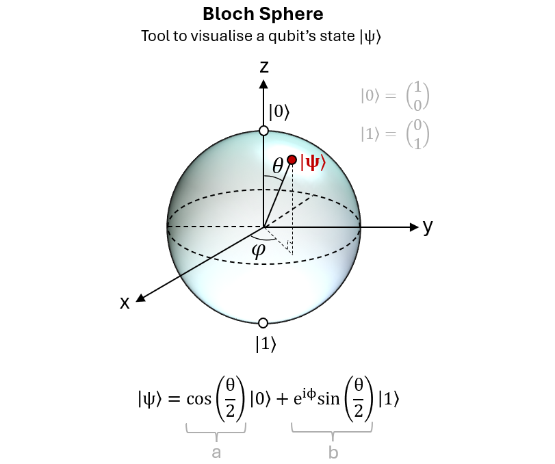
To solidify this concept, let's watch a short video explaining this mapping and then read a concise article that puts the two equations side-by-side.

Now, let's see this in writing. The following resource concisely shows the transformation from the a and b form to the θ and φ form.

3. Exploring Key States on the Bloch Sphere

Let's use this new representation to explore some important qubit states and build our intuition.

• State |0⟩: To get this state, we need the |1⟩ component to be zero. This happens when sin(θ/2) = 0, which means θ/2 = 0, so θ = 0. This places the state vector at the North Pole.

• State |1⟩: Here, we need the |0⟩ component to be zero. This happens when cos(θ/2) = 0, which means θ/2 = π/2, so θ = π. This places the state vector at the South Pole.

• State |+⟩ = (|0⟩ + |1⟩)/√2:
  This is an equal superposition. The coefficients are 1/√2 for both |0⟩ and |1⟩.

  • cos(θ/2) = 1/√2 => θ/2 = π/4 => θ = π/2. This puts the state on the equator.
  • e^(iφ)sin(θ/2) = 1/√2. Since sin(π/4) = 1/√2, we need e^(iφ) = 1. This occurs when φ = 0.
  • This state points along the positive x-axis.

• State |i⟩ = (|0⟩ + i|1⟩)/√2:

  • cos(θ/2) = 1/√2 => θ = π/2. Again, on the equator.
  • e^(iφ)sin(θ/2) = i/√2. We need e^(iφ) = i. This occurs when φ = π/2.
  • This state points along the positive y-axis.

The Bloch sphere gives us a fantastic geometric picture. Applying a quantum gate to a qubit is equivalent to performing a rotation of its state vector on the surface of this sphere. We'll explore this in detail in the next module.

Conclusion

In this lesson, we have put the mathematical structure behind our conceptual model of a qubit.

Key Takeaways:

• Dirac notation is a shorthand for describing quantum state vectors. The "ket" |ψ⟩ represents a column vector.
• The general state of a single qubit, |ψ⟩ = α|0⟩ + β|1⟩, can be written as the vector [α, β]ᵀ.
• The Bloch sphere provides a geometric representation of a single-qubit state.
• Any single-qubit state can be parameterized by two real angles, θ and φ, and represented as a point on the sphere's surface:
  $|\psi ⟩=\cos (\frac{\theta }{2})|0⟩+e^{i\varphi }\sin (\frac{\theta }{2})|1⟩$
• The poles of the sphere represent the classical basis states (|0⟩ and |1⟩), while points on the equator represent equal superpositions. The longitude (φ) represents the relative phase.

Preview of the Next Lesson:
We now have a complete representation of a qubit's state. But what happens when we want to get information out of it? In the next lesson, we will address the final piece of the single-qubit puzzle: measurement. We will learn how to calculate the probabilities of measurement outcomes from a given single-qubit state vector, connecting the amplitudes α and β directly to what we observe in an experiment.