Quantum Measurement Probabilities

1. The Born Rule: From Amplitudes to Probabilities

The complex numbers α and β in the state vector |ψ⟩ = α|0⟩ + β|1⟩ are called probability amplitudes. They are not probabilities themselves, but they contain all the information needed to find the probabilities.

The rule that connects them is called the Born Rule. It states that the probability of measuring a specific classical state is the squared magnitude (or absolute value squared) of its corresponding amplitude.

For a single qubit, this is very straightforward:

• The probability of measuring the outcome 0 is $P(0)=|\alpha {|}^2$.
• The probability of measuring the outcome 1 is $P(1)=|\beta {|}^2$.

Since probabilities must be real, non-negative numbers, taking the squared magnitude makes perfect sense. For a complex number $z=a+bi$, its squared magnitude is $|z{|}^2=a^2+b^2$, which is always real and non-negative.

Let's watch a clip that explains this process of measurement clearly.

As the video explains, this rule is a core postulate of quantum mechanics—we accept it because it perfectly describes what we observe in experiments.

2. The Normalization Constraint

You know from basic probability theory that if you have a complete set of possible outcomes, their probabilities must sum to 1. In our case, measuring a qubit in the computational basis can only yield a 0 or a 1. Therefore, it must be true that:

$P(0)+P(1)=1$

Substituting the Born Rule into this equation gives us the normalization condition that we've seen before:

$|\alpha {|}^2+|\beta {|}^2=1$

This constraint ensures that our state vector always corresponds to a valid probability distribution. Geometrically, it means the vector representing the quantum state must have a length (or Euclidean norm) of 1.

The following video offers a simple, powerful analogy for this constraint.

This unit circle is a 2D projection of the 3D Bloch sphere, tying the geometric picture back to the probabilistic nature of measurement.

3. Step-by-Step Probability Calculations

Let's put this into practice with a few examples.

Example 1: Equal Superposition

Consider the |+⟩ state we've seen before:
$|+⟩=\frac{1}{\sqrt{2}}|0⟩+\frac{1}{\sqrt{2}}|1⟩$
Here, $\alpha =\frac{1}{\sqrt{2}}$ and $\beta =\frac{1}{\sqrt{2}}$.

• Probability of measuring 0:
  $P(0)=|\alpha {|}^2={\left|\frac{1}{\sqrt{2}}\right|}^2=\frac{1}{2}=50\%$
• Probability of measuring 1:
  $P(1)=|\beta {|}^2={\left|\frac{1}{\sqrt{2}}\right|}^2=\frac{1}{2}=50\%$

This makes intuitive sense: a state in an equal superposition of |0⟩ and |1⟩ should have a 50/50 chance of being measured in either state.

Example 2: A State with Complex Amplitudes

Now let's take a state with a complex phase:
$|\psi ⟩=\frac{1}{2}|0⟩+\frac{\sqrt{3}i}{2}|1⟩$
Here, $\alpha =\frac{1}{2}$ and $\beta =\frac{\sqrt{3}i}{2}$.

• Probability of measuring 0:
  $P(0)=|\alpha {|}^2={\left|\frac{1}{2}\right|}^2=\frac{1}{4}=25\%$
• Probability of measuring 1:
  $P(1)=|\beta {|}^2={\left|\frac{\sqrt{3}i}{2}\right|}^2={\left(\frac{\sqrt{3}}{2}\right)}^2=\frac{3}{4}=75\%$

Notice how the imaginary number i disappears when we take the magnitude. The phase of an amplitude does not affect the measurement probabilities in this basis, but as we'll see later, it's crucial for interference effects and the behavior of quantum algorithms.

Your Turn: Practice Calculation

Now it's your turn. Let's use an exercise from an IBM Qiskit learning module to test this.

The state given is $|\psi ⟩=\sqrt{\frac{3}{5}}|0⟩+\sqrt{\frac{2}{5}}|1⟩$.

• What is the probability of measuring |0⟩?
• What is the probability of measuring |1⟩?

After calculating, check your answers against the solution provided in the resource. You should find $P(0)=3/5=60\%$ and $P(1)=2/5=40\%$.

4. Measurement in Practice: Collapse and Statistics

The probabilities tell us the likelihood of an outcome, but what happens when a measurement is actually performed?

1. A single measurement is definitive: If you measure a single qubit in the state $|\psi ⟩=\sqrt{0.6}|0⟩+\sqrt{0.4}|1⟩$, you will get either 0 or 1. You will never get "60% of a 0." The quantum state's superposition is resolved into a single classical outcome.
2. State Collapse: The act of measurement fundamentally alters the state. If you measure the qubit and get the outcome 0, the qubit's state is no longer |ψ⟩; it has collapsed to |0⟩. A subsequent measurement will now yield 0 with 100% certainty (ignoring hardware noise).
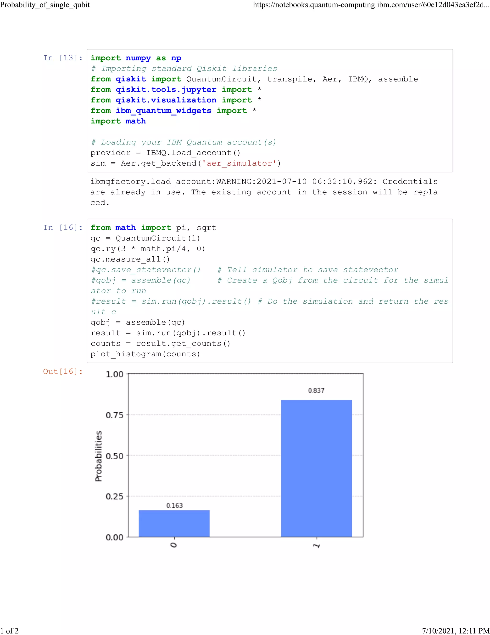
3. Probabilities emerge from statistics: The probabilities we calculate only become apparent when we repeat the experiment many times on identical copies of the state |ψ⟩. If you prepare and measure this state 1000 times, you will find the outcome is 0 approximately 600 times and 1 approximately 400 times.

This is exactly what we see when we run simulations in Qiskit. The simulator calculates the probabilities and then uses them to randomly sample outcomes for the number of "shots" (repetitions) you request. The result is a histogram of counts.

Conclusion

Today, we've unlocked the connection between the abstract state vector and the concrete results of a quantum measurement. This is the mechanism that allows us to extract answers from a quantum computer.

Key Takeaways:

• The Born Rule is the principle that allows us to calculate measurement probabilities from a quantum state.
• For a state $|\psi ⟩=\alpha |0⟩+\beta |1⟩$, the probability of measuring 0 is $P(0)=|\alpha {|}^2$ and the probability of measuring 1 is $P(1)=|\beta {|}^2$.
• The normalization condition, $|\alpha {|}^2+|\beta {|}^2=1$, ensures that the probabilities sum to one.
• A single measurement gives a definite outcome (0 or 1) and collapses the quantum state to the corresponding basis state.
• The calculated probabilities are revealed statistically by repeating the measurement on many identical states.

Preview of the Next Module:
This concludes our foundational module. We now have a complete picture of a single qubit: how to represent its state and how to predict its measurement outcomes. In the next module, "Manipulating Qubits with Quantum Gates," we will finally start performing computations. We will learn how to apply operations—quantum gates—that systematically rotate the state vector on the Bloch sphere, changing its amplitudes α and β, and thus controllably altering the measurement probabilities to solve problems.