Welcome! In our last lesson, we focused on how to interpret and visualize the results of a quantum simulation using histograms. You learned to transform a dictionary of measurement counts into an intuitive plot that reveals the probabilistic nature of a quantum circuit.
Today, we will put all the pieces from the last few lessons together. We will perform a complete, end-to-end "quantum experiment" on a simulator. Our goal is to build and simulate a Bell state circuit in Qiskit and use the results to verify the presence of quantum entanglement. This is a milestone in your quantum computing journey, as you'll be creating and confirming one of the most famous and foundational states in the field.
1. Understanding Entanglement and Bell States
Before we start coding, it's crucial to have a solid conceptual understanding of what we're trying to create. A Bell state is a special state of two qubits that are maximally entangled. Entanglement is a type of correlation between quantum particles that is stronger than any possible classical correlation. Einstein famously called it "spooky action at a distance." In an entangled state, the properties of the qubits are linked, regardless of the distance separating them. Measuring one qubit instantly influences the outcome of the other.
The following video from the Qiskit channel provides an excellent, non-mathematical explanation of entanglement and introduces the Bell states.
This video explains the core concept of entanglement and introduces the Bell states.
First, watch the introduction to understand how quantum correlation differs from classical correlation. Then, watch the section that defines entangled states and the four Bell states. Pay close attention to the description of the Φ+ (Phi-plus) state, as this is the one we will create. Notice the key property: if you measure one qubit as 0, the other is guaranteed to be 0, and if you measure it as 1, the other is guaranteed to be 1.
The specific Bell state we'll create is the |Φ⁺⟩ (Phi-plus) state, which is an equal superposition of the |00⟩ and |11⟩ states. Its state vector is written as:
This equation tells us there's a 50% probability of measuring the state as 00 and a 50% probability of measuring it as 11. Crucially, the probability of measuring 01 or 10 is zero. This perfect correlation is the signature of entanglement we will look for in our simulation.
2. Building the Bell State Circuit in Qiskit
Now, let's build the circuit that generates this state. The process involves just two gates:
- Hadamard (H) gate: Applied to the first qubit to put it into a superposition of
|0⟩and|1⟩. - Controlled-NOT (CNOT) gate: Applied with the first qubit as the control and the second as the target. This creates the entanglement.
This is the standard recipe for creating a Bell state. Here is what the final circuit looks like:

The following tutorial provides a complete, step-by-step walkthrough for creating and simulating this circuit. We will work through it together.
Getting Started with Qiskit: Basics Quantum Circuit
This article will guide you through the entire process, from setting up the environment to visualizing the final results.
Please read through the article starting from section "1.3 Setting up Colab Environment" to the end. As you read, follow the steps to write and execute the code in your own Qiskit notebook. Here's a breakdown of the key stages in the article: Environment Setup: The article mentions installing Qiskit. You should already have this set up, but it's a good reminder. Circuit Creation (1.4 Your First Quantum Circuit): Follow the code to import QuantumCircuit, initialize a circuit with 2 qubits and 2 classical bits, and then add the h() and cx() gates. The article does a great job explaining how each gate transforms the state. Visualization (1.5 Visualizing Your Circuit): Use qc.draw('mpl') to see the circuit you've just built. Does it match the diagram shown above? Simulation (1.6 Simulating Quantum Circuits): This is the execution step. The code shows you how to import AerSimulator, transpile the circuit (a good practice for optimizing it for a backend), and run the simulation for 1024 "shots." Interpreting Results: Finally, the article shows you how to get the counts dictionary and, most importantly, use plot_histogram to visualize the outcomes.
3. Verifying Entanglement from the Simulation
After running the code from the tutorial, you should see a histogram displayed as the output. It will look very similar to this:
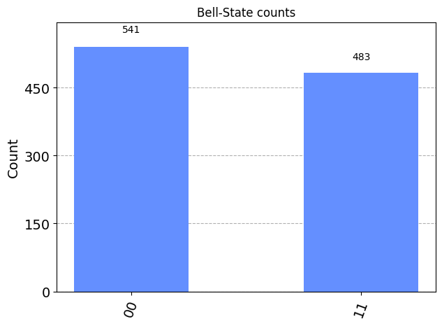
Now, let's analyze this result. This is the "verification" step.
- What outcomes do you see? You should only see bars for the
'00'and'11'states. - What outcomes are missing? The states
'01'and'10'should have zero (or near-zero) counts. - What does this mean? The absence of the mixed states
'01'and'10'is the experimental proof that our qubits are entangled. Their measurement outcomes are perfectly correlated. If the first qubit is measured as 0, the second is always 0. If the first is 1, the second is always 1. You can't describe the state of one qubit independently of the other, which is the very definition of entanglement.
Congratulations! You have successfully built an entangled state and verified its properties through simulation.
4. Further Exploration (Optional)
You've now mastered the creation of the |Φ⁺⟩ state. There are actually four Bell states in total, each representing a different form of maximal entanglement. They can all be created with minor variations of the circuit you just built.
Introduction to Bell states in Qiskit with Code
This tutorial from Quantum Computing UK introduces all four Bell states and provides the circuits and code to create them.
Start by looking at the "What are Bell states?" section to see the definitions of all four states (|Φ⁺⟩, |Φ⁻⟩, |Ψ⁺⟩, and |Ψ⁻⟩). Then, skip to the diagrams showing the circuits for the second, third, and fourth Bell states. Notice how they are constructed by adding simple Pauli-X or Z gates to our original circuit. Finally, you can look at the full Python code at the end of the article, which contains functions for generating all four states. You can try running this code to see the different measurement outcomes for each state.
This optional exercise is a great way to solidify your understanding and see how a small change in the circuit can lead to a completely different (but still entangled) final state.
Conclusion
In this lesson, you consolidated your Qiskit skills to perform a complete quantum simulation from start to finish. You have moved from theory to practice, demonstrating one of the most counter-intuitive yet powerful features of quantum mechanics.
Key Takeaways:
- A Bell state is a maximally entangled two-qubit state where the measurement outcomes are perfectly correlated.
- The standard circuit to create a
|Φ⁺⟩Bell state uses a Hadamard gate followed by a CNOT gate. - Entanglement is verified by simulating the circuit and observing the measurement results. For
|Φ⁺⟩, the absence of|01⟩and|10⟩outcomes in the histogram confirms the correlation. - You have successfully completed an end-to-end workflow: defining a quantum state, building a circuit to create it, simulating it, and analyzing the results to verify its properties.
Preview of the Next Lesson:
We have seen that when we measure a qubit in superposition, it "chooses" a definite classical state (0 or 1). In the next lesson, "Explain how measurement collapses a quantum superposition into a definite classical state," we will explore this process of measurement itself more deeply. We'll discuss what "collapse" means and its profound implications for quantum computation.