Simulating Quantum Circuits with Qiskit Aer

1. The Role of Simulators and Qiskit Aer

Before we run a circuit on a real, multi-million dollar quantum computer, we almost always simulate it first. Simulators are essential tools for several reasons:

• Ideal Environment: They provide a perfect, noiseless world where your qubits behave exactly as the mathematics predicts. This is crucial for learning algorithms and debugging your code without the complexities of hardware errors.
• Accessibility: You can run simulations on your own laptop anytime, without waiting in a queue for access to real hardware.
• Specialized Insights: Simulators can provide information that is impossible to get from a real device, such as the full quantum state vector of your circuit at any point in the computation.

Qiskit Aer is IBM's open-source, high-performance simulation package. It's written in C++ for speed and provides several different simulation backends tailored for various tasks.

The video below explains why Aer is so powerful, particularly for circuits with many qubits where efficiency becomes critical.

2. The Simulation Workflow: From Circuit to Counts

Let's take the Bell state circuit you built in the last lesson and run it through a simulation. The goal is to verify that we get the expected outcome: a 50/50 probability of measuring 00 or 11.

The process involves four main steps:

1. Build the Circuit with Measurements: We add measurement operations to map the final quantum state of the qubits to classical bits.
2. Choose and Instantiate a Simulator: We select the AerSimulator.
3. Run the Simulation: We execute the circuit on the simulator for a specific number of "shots".
4. Get the Results: We retrieve the aggregated measurement outcomes, called "counts".

The following reading walks through this exact workflow. We'll break it down step-by-step.

Let's implement this together in your own notebook.

Step 1: Build the Circuit and Add Measurements

First, we reconstruct our Bell state circuit. Crucially, we must also tell Qiskit what to measure and where to store the results. We do this by adding .measure_all(), which adds a measurement operation to each qubit and stores its result in a corresponding classical bit.

from qiskit import QuantumCircuit




# Create a circuit with 2 qubits and 2 classical bits
qc = QuantumCircuit(2, 2)




# 1. Put qubit 0 into superposition
qc.h(0)




# 2. Entangle qubit 1 with qubit 0
qc.cx(0, 1)




# 3. Add measurements
qc.measure([0, 1], [0, 1])




# Draw the final circuit
qc.draw("mpl")

You will see measurement symbols at the end of your circuit, indicating the final quantum state is being read out into the classical bits.

Step 2: Choose the Simulator

As the reading explains, we import and create an instance of the AerSimulator. This object represents the virtual quantum computer we'll run our circuit on.

from qiskit_aer import AerSimulator




# Create an instance of the simulator
simulator = AerSimulator()

Step 3: Run the Simulation

Now we execute the circuit. Quantum mechanics is probabilistic, so a single run doesn't tell us much. We must repeat the experiment many times to build up statistics about the outcomes. Each repetition is called a shot.

The simulator.run() method takes our circuit and the number of shots as arguments. It returns a Job object, which is a handle to our simulation task.

# Run the simulation for 1024 shots
job = simulator.run(qc, shots=1024)

Step 4: Get the Results

The job object contains the results of our simulation. We retrieve them using the .result() method. From the result object, we can get a dictionary of the measurement outcomes using .get_counts().

# Get the result from the job
result = job.result()




# Get the counts dictionary
counts = result.get_counts(qc)

print("Measurement outcomes:", counts)

You should see an output similar to this:
Measurement outcomes: {'00': 518, '11': 506}

The keys of the dictionary ('00', '11') are the classical bitstrings that were measured, and the values are the number of times each outcome occurred out of 1024 shots. As expected, the outcomes 01 and 10 do not appear, and the counts for 00 and 11 are roughly equal. The slight deviation from a perfect 500/500 split is due to the statistical nature of quantum measurement, similar to how flipping a fair coin 1000 times won't give you exactly 500 heads and 500 tails.

3. Simulator Backends and Noise

The AerSimulator is highly versatile. It can operate using different mathematical methods, or "backends," optimized for certain types of circuits. It can also simulate the noise and errors present in real quantum hardware.

This ability to model noise is critical for developing error-correction techniques, a topic we'll explore in the final module. For now, we will continue to use the default ideal simulator.

The different simulation methods within Aer (e.g., statevector, matrix_product_state) are advanced options that offer performance trade-offs. For most common circuits, the default automatic method is sufficient.

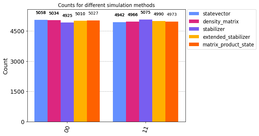
This is analogous to choosing different numerical solvers in an engineering simulation tool; you have options, but they all aim to solve the same underlying physical model.

Conclusion

In this lesson, you've bridged the gap between designing a quantum circuit and seeing its results. You learned how to use Qiskit Aer, a powerful simulation engine, to execute your circuits and interpret the probabilistic outcomes. This simulation step is fundamental to the entire field, serving as the primary tool for developing, testing, and understanding quantum algorithms before they are ever sent to real hardware.

Key Takeaways:

• Simulators are essential for learning and debugging quantum algorithms in an ideal, noiseless environment.
• Qiskit Aer is a high-performance simulation toolkit for Qiskit.
• The simulation workflow involves building a circuit with measurements, instantiating a simulator, running the job with shots, and retrieving the counts.
• Shots are repetitions of the experiment needed to build up statistics for the probabilistic outcomes.
• The .get_counts() method returns a dictionary where keys are the measured bitstrings and values are the number of times they occurred.

Preview of the Next Lesson:
We've successfully obtained the raw counts data from our simulation. While a dictionary of numbers is useful, a visual representation is often more insightful. In the next lesson, we will learn how to use Qiskit's visualization tools to create histograms from our simulation results, allowing us to see the probability distribution of outcomes at a glance.